Blog · Structured light ·
From two rays to a point cloud: triangulation by the sine rule
Two rays, a known baseline, a triangle. The scanner derives depth from the law of sines instead of the usual least-squares midpoint. Then the messy real part: voxel downsampling, bounding-box cropping, and reading a mirror-image ghost handle back to its cause.
- interactive
- structured-light
- computer-vision
- triangulation
- point-cloud
- webgl
This is the payoff of a four-post chain. Post 40 labels every projector column and row with a Gray code. Post 49 turns a laptop and a phone into a rig that photographs the labels. Post 51 (not yet published as I write this, see the widget note below) decodes those photographs, pixel by pixel, into a projector column and row for every camera pixel it trusts. None of that is a 3D point yet: it’s two 2D coordinate systems agreeing on where a point is, without saying how far away it is. This post is the last mile: turn a camera ray and a projector ray that look at the same point into that point’s actual position, over however many hundred thousand pixels the camera has.
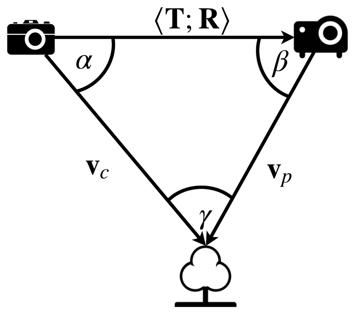
Report Fig. 1, p.5, the same diagram post 40 opened with. and are the rays from camera and projector to the same object point; is the rigid transform between them, found once by calibration and reused for every point.
The sine rule, not the midpoint
The standard way to triangulate two rays that (in theory) meet at a point is least-squares: the
rays are almost never exactly coplanar once there’s any pixel-location noise, so you find the
3D point that minimises the sum of squared distances to both rays: cv2.triangulatePoints
does this, and it’s what most stereo pipelines reach for, including this site’s own
epipolar geometry post. This project’s own reconstruction code
does something else. It treats the camera ray, the projector ray and the baseline between them
as a triangle and solves it with the law of sines, taking the camera ray as authoritative rather
than splitting the difference between two rays that may not actually intersect.
Report §2 sets up the two equations (p.5, Eqs 2.1–2.2). The angles come from the dot product,
and once two angles of the triangle are known, the third follows because the interior angles of a triangle sum to , and the sine rule gives the missing side:
where is the angle at the camera (between the baseline and the camera ray), is the angle at the projector, and is the angle at the object point itself, the angle between the two rays, which is also exactly the thing that goes wrong when a scene point is far away: a distant point makes shrink toward zero, the classic narrow-baseline stereo problem. is the length of the side opposite , which is the camera-to-object distance. Multiply the unit camera ray by and you have the point.
Reading the code
The whole thing, vectorised over every valid pixel in one scan, lives in the reconstruction script:
LPts = cv2.convertPointsToHomogeneous(cv2.undistortPoints(indImg1[None,], cameraMatrix1, distCoeffs1, R=R))[:,0].T
RPts = cv2.convertPointsToHomogeneous(cv2.undistortPoints(indImg2[None,], cameraMatrix2, distCoeffs2))[:,0].T

TLen = np.linalg.norm(T)
NormedL = LPts/np.linalg.norm(LPts, axis=0)
alpha = np.arccos(np.dot(-T, NormedL)/TLen)
degalpha = alpha*180/np.pi
beta = np.arccos(np.dot(T, RPts)/(TLen*np.linalg.norm(RPts, axis=0)))
degbeta = beta*180/np.pi
gamma = np.pi - alpha - beta
P_len = TLen*np.sin(beta)/np.sin(gamma)
Pts = NormedL*P_len
indImg1 is every trusted camera pixel (u, v); indImg2 is the projector (column, row)
post 51’s decode put there. cv2.undistortPoints turns a pixel into a normalised ray: divide
out the intrinsics, correct the lens distortion, and you have a direction with . The
R=R argument on the camera side is doing something specific: undistortPoints accepts a
rectification rotation and applies it to the ray it returns, so LPts isn’t the camera ray in
the camera’s own frame. It’s the camera ray rotated into the projector’s frame by the same
R that calibration produced (X_\text{proj} = R\,X_\text{cam} + T, the cv2.stereoCalibrate
convention this project’s calibration step uses, and the R that Eqs 2.1–2.2 call
). RPts is the projector ray in its own frame: no
rotation needed, it’s already there. This is why alpha and beta come out right despite being
computed from vectors nominally in different frames going in: the angle between two vectors
doesn’t change if you rotate both of them by the same rotation, and T, NormedL and RPts
have all, one way or another, ended up expressed in the projector’s frame.
A subtlety I chose not to reproduce
Pts = NormedL * P_len scales the (rotated) camera ray by the computed distance and stops
there: it never adds T. If the whole triangle really is being solved in the projector’s
frame, the object point should be the projector’s view of the camera’s origin, plus the ray:
T + P_len * NormedL, because the ray starts at the camera, and the camera’s origin sits at T
once you’re looking from the projector’s frame. Omitting it doesn’t distort the cloud. Every
point gets the same missing offset, so it’s a rigid translation of the “correct” one, invisible
in a bare point-cloud render and irrelevant to every distance-based figure in the report (the
Kinect comparison in §7.3 registers the two clouds with ICP anyway, which absorbs any constant
offset). It does mean my own point cloud isn’t actually anchored at the camera, and the report
doesn’t say so either.
Porting it to Rust
Post 51 already built the WASM crate that decodes the images, and its documented output format:
real projector pixel indices per axis, plus a 2-bit invalid mask, one bit per axis, row-major
over the working resolution. This post doesn’t touch that crate’s decoder; it adds one new
module for the triangulation kernel, wired in with a single pub mod triangulate; line in the
crate’s root. The kernel itself is close to what I expected going in: about ten lines of real
trigonometry once you strip the plumbing:
let gamma = PI - alpha - beta;
if !(gamma > min_gamma_rad) || !(gamma < PI - min_gamma_rad) || !gamma.is_finite() {
    return invalid;
}
let d = t_len * beta.sin() / gamma.sin();
if !(d.is_finite() && d > 0.0) {
    return invalid;
}
Tri { p: scale3(rc, d), valid: true }
min_gamma_rad is the guard the plain sine rule doesn’t have: as a point recedes, and , and in the denominator is happy to turn any leftover
floating-point noise in into a depth of a few hundred kilometres. Rejecting a
near-parallel pair outright, rather than returning whatever d falls out, is the difference
between a stray point flying off into the distance and the widget saying “don’t know.”
Six automated tests cover it: the sine rule recovers a known synthetic depth
to within 0.05 mm; a deliberately near-parallel ray pair (an object placed two million millimetres
out) is rejected rather than returning a huge ; a triangulated point reprojects back onto its
exact source camera pixel (true to floating-point precision, since the point is constructed as
d * (camera ray), this one is really just checking the algebra didn’t get scrambled somewhere);
and voxel downsampling both reduces the point count and keeps every output point inside the
input’s bounding box. The crate compiles to 31.6 kB (shared with post 51’s decoder, which is most
of it; this module’s own kernels are a few hundred lines). Timed directly in a browser against
1,000,000 synthetic points: tri_triangulate runs in 67 ms and the voxel-grid downsample (2 mm
buckets, reducing to 334,299 points) in 144 ms. Both single WASM calls, no allocation inside the
hot loop. The widget’s own working resolution is much smaller (480×340, 163,200 points), so the
same two calls complete in well under 20 ms there, which is what makes dragging the baseline
slider live rather than debounced.
The messy real part
A triangulated cloud straight off the sine rule is much denser than it needs to be, because the
camera out-resolves the projector: the report’s Canon shoots 5184×3456, its projector is
1024×768, roughly five camera pixels per projector pixel along each axis. Every one of those
camera pixels that decodes to the same projector column and row produces its own 3D point, at
a very slightly different depth (sub-pixel decode noise), so a flat surface comes out as a comb
of near-duplicate points rather than a single sheet. Open3D’s voxel_down_sample, called on the
raw cloud right after triangulation, before anything else happens to it, buckets points into a
grid at a chosen voxel_size (0.5 mm in the report) and replaces every occupied cell with the
centroid of whatever fell into it. The Rust port’s tri_voxel_downsample does the same
bucket-and-average, implemented with a hash map keyed on the floored voxel coordinate rather
than a spatial tree. Simpler, and fast enough at these point counts.
After that, a hard-coded bounding box throws away everything outside the scanning volume:
filterLocs = np.logical_and(np.logical_and(pts_hold[:, 2] < 950, pts_hold[:, 2] > 200),
                            np.logical_and(np.logical_and(pts_hold[:, 0] < 530, pts_hold[:, 0] > -60),
                                           np.logical_and(pts_hold[:, 1] < 160, pts_hold[:, 1] > -350)))
Six numbers, tuned by hand for the report’s rig and never explained beyond “remove artefacts in
the background and shift the focus to the object which is currently being scanned” (§4.2.4).
Colour comes along for the ride: img[indImg1[0], indImg1[1]] reads straight off the fully-lit
reference photograph at the same camera pixel, so the point cloud is coloured by an ordinary
photograph, not by anything structured-light-specific.
Reading the artefacts back to their causes
None of this is free of errors, and the report does not hide where they come from (§7.2). A few, read straight off Figs. 12–14:
- The shadow under the object is invalid, not wrong. Post 51’s classifier marks a shadowed pixel “uncertain” rather than guessing: exactly the shadow-cast band you’d expect behind an object lit from one side by the projector. That’s the whole point of the third answer: the cloud has a hole there instead of a plausible-looking lie.
- A mirror-image ghost of the handle sticks out toward the camera. The report traces this to a real reflection: “the reflective surface placed underneath the objects created a near-mirror image of some of the objects in the point clouds.” Light bouncing off a shiny surface confuses the classifier into reporting a confident, wrong correspondence, which triangulates into a real-looking point in entirely the wrong place. Unlike the shadow, this isn’t caught, because nothing about a specular reflection makes the decoder doubt itself.
- Dark surfaces vanish outright: Fig. 13’s “hole-punch” scene classifies as almost entirely uncertain, because the threshold (post 51’s reliability floor on ) can’t be met when the surface barely reflects anything back.
- Errors cluster at silhouette edges, where the projected pattern is compressed by a sudden depth discontinuity and a few camera pixels straddle a boundary the decode can’t resolve cleanly. Small, and mostly cropped away by the bounding box.
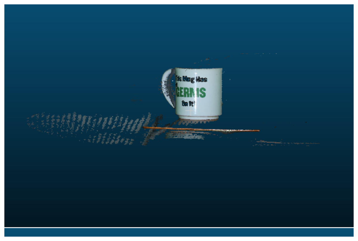
Report Fig. 14 (top), p.23: the real “Cup” scene, projector-camera reconstruction. This is a real capture from the report; the widget below reconstructs a synthetic scene, not this one. See “what the widget is actually showing you” below.
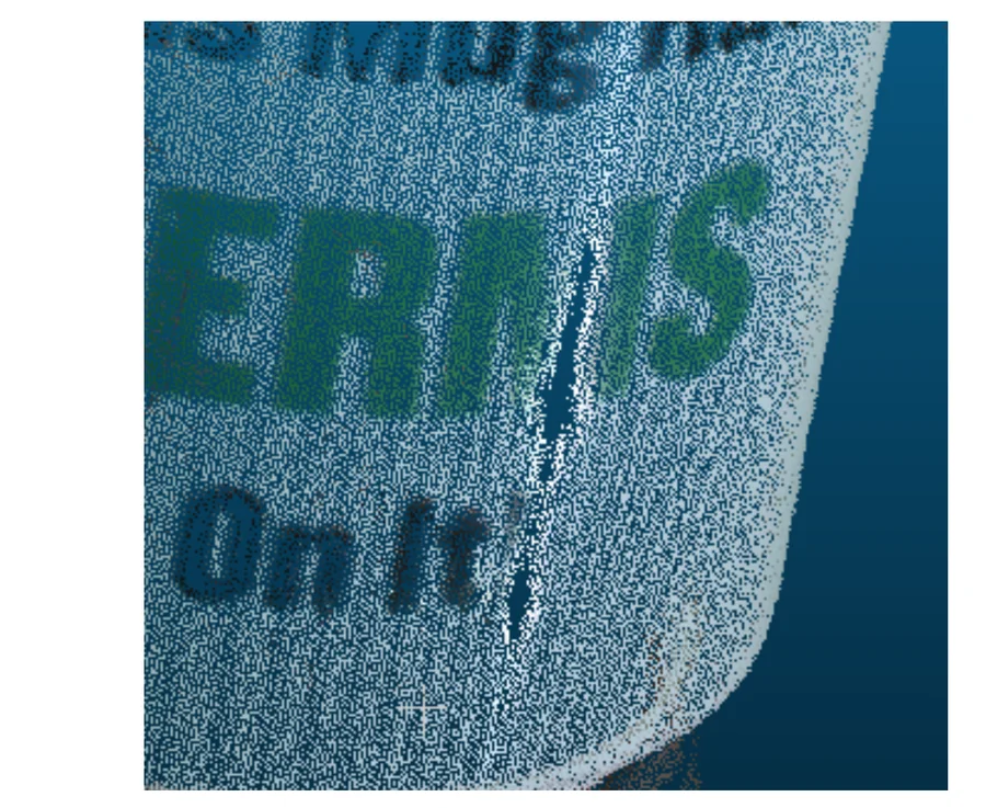
Report Fig. 14 (detail), p.23. Dense enough, and accurate enough, that printed text on the mug is legible in the raw point positions: this is the reconstruction’s actual resolution, not an illustration.
The Kinect, for comparison
The report runs a second, independent reconstruction of the same scenes with a Kinect for Xbox 360, mounted alongside the camera. It’s not structured light in the Gray-code sense, the Kinect projects its own fixed infrared dot pattern and reads depth off a single exposure, but it gives an independent measurement to check the sine-rule cloud against. The Kinect reconstruction script deliberately doesn’t use OpenNI’s own depth-to-point-cloud conversion:
In other words, OpenNI’s own reprojection assumes an undistorted lens, and the actual IR sensor isn’t
one, so the report calibrates it properly, with the same ChArUco pipeline as the main camera,
and reprojects by hand: undistort each pixel into a ray, scale by
the depth reading, then cv2.projectPoints the result into the RGB camera’s frame to pick up
colour. Same shape of problem as the main pipeline, different sensor.
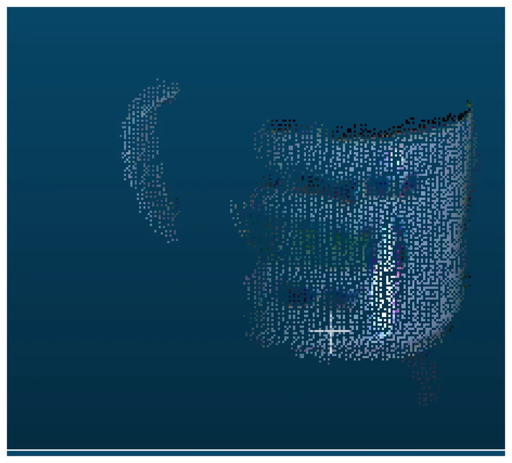
Report Fig. 15, p.24: the same “Cup” scene, Kinect reconstruction. Compare directly against Fig. 14 above: same mug, same table, same camera framing.
The contrast is the point. The projector-camera cloud resolves printed text on a mug; the Kinect gives a recognisably mug-shaped blob and nothing finer, which the report attributes plainly to what the sensor is actually designed for:
And yet, once the two clouds are registered (by hand, in CloudCompare, not something this project automated), they largely agree:
That’s the actual accuracy claim in this report: not a synthetic benchmark, but two independently built 3D sensors, calibrated separately, agreeing to within about two millimetres on most of a scene. Sub-2mm agreement between a $50 hobbyist rig and a commercial depth camera is a genuinely good result for a university project.
Colour, three ways
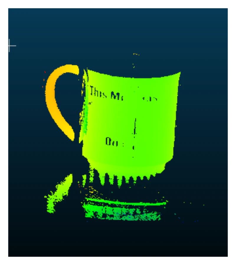
Report Fig. 16, p.25, CloudCompare’s height-ramp colouring, height mapped through a colour gradient. Useful for reading depth structure that photographic colour hides.
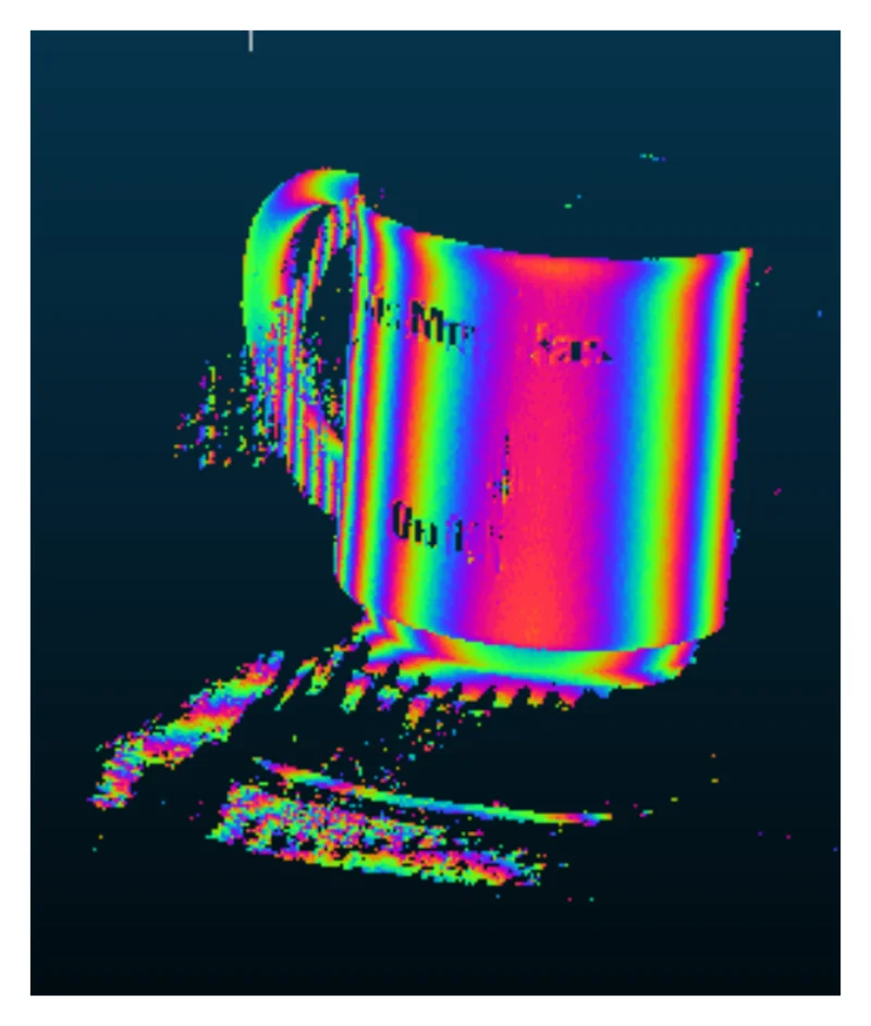
Report Fig. 17, p.25, the same view, banded every 10 mm instead of ramped continuously. The bands read almost like contour lines on the mug’s curved surface, a cheap, effective way to see curvature that a photograph can’t show.
Both are CloudCompare features applied after the fact to the same cloud Fig. 14 shows; nothing in
this project’s own code produces them. The widget below reproduces both as live shader colour
modes, alongside the plain photographic colouring the reconstruction script actually writes to the .ply.
The octree coda (a footnote, not a section)
The report’s final step feeds the cropped, filtered cloud into OctoMap, an occupancy-grid octree
that repeatedly halves space and only subdivides where points actually are, a good fit for
collision detection and for compressing a point cloud that has a lot of near-duplicate points
close together (Table 2, p.36: the “Cup” scene goes from 4716 points to a 164 KB .bt file).
The script that drives it is seventeen lines, and every one of them is either a path or a
subprocess.call:
subprocess.call([octomap_exe_path, ftp, outpath+file+".bt"])octomap_exe_path points at a prebuilt Windows binary that isn’t included in the repository,
reached through a hardcoded path that assumes a particular local build tree. There’s no
algorithm here to port, quote, or reimplement; it’s a shell-out to a tool the report used and
didn’t ship. Worth knowing the report’s pipeline has this last step, not worth a section, and
not something the widget below attempts.
Try it: triangulate and orbit
Drag the baseline slider and watch the cloud stretch along : a shorter baseline makes (the angle between the two rays at the object) shrink faster with depth, so the same pixel-location noise in and turns into a larger depth error; the report’s real rig used about 264 mm for exactly this reason, an offset large enough to keep comfortable across the scanning volume without making the projector’s field of view stop overlapping the camera’s. The calibration panel is pre-filled with the report’s real , , and (p.22); every field is editable.
With JavaScript on, this becomes a live WebGL point-cloud reconstruction: an editable calibration panel, a baseline scrubber, a voxel-size slider with a live point count, six bounding-box crop planes, three colour modes, a “show discarded” overlay for the pixels the decode gave up on, and a .ply download. Without it, here’s an orbit of one of the report’s own real reconstructions (re-encoded from the report’s original 12 MB animated GIF of the same orbit).
Rendering is a single hand-rolled WebGLRenderingContext: one vertex shader, one fragment
shader, one gl.POINTS draw call. A point cloud is close to the simplest thing WebGL is for:
there’s no scene graph, no material system, no lighting model worth the name, so three.js (an option I considered for this post) would
mostly be dead weight here. Every other widget on this site
is dependency-free, and this one had no real reason to be the exception. The vertex shader does
more than place points: bounding-box cropping, height-ramp and banded colour selection, and the
discarded-point overlay are all uniform-driven branches inside it, so dragging a bounding-box
slider or flipping colour mode is a uniform update and a redraw: no CPU-side buffer rebuild,
which is what keeps those controls smooth. Baseline and voxel-size changes do rebuild the GPU
buffers, because the point positions actually change; both round-trip through the WASM kernels
above and stay comfortably under a frame budget at this working resolution (480×340, capped well
under the ~2M-point ceiling I set for this post, a deliberate scope cut given the scene is
synthetic, not a real multi-megapixel capture).
Orbit with a pointer drag, the mouse wheel to zoom, or (since a canvas has no keyboard semantics
of its own) arrow keys and +/− once it has focus. It doesn’t orbit on its own: the auto-orbit
checkbox is the only motion that isn’t a direct response to input, it’s unchecked by default, and
it’s disabled entirely under prefers-reduced-motion.
What this closes out
Four posts, one working instrument: generate patterns → capture a bundle → decode it (post 51) → reconstruct it, entirely in a browser, no server. The maths in this last step is genuinely small (a triangle, the law of sines, a voxel grid), which is exactly why it’s worth taking seriously: the hard parts of a structured-light scanner are deciding what to trust (post 51) and getting a camera and a projector to agree on a coordinate system at all (the calibration posts this series doesn’t cover here); once both of those are done, turning two agreeing pixels into a point is almost an afterthought, and the report’s own code proves it in thirteen lines.