Support vectors: why only a handful of your data points matter

The report this comes out of opens Part A by contrasting two kinds of model. A parametric one fits a fixed set of weights and then the training data can be discarded; a kernel method keeps the training data around, because prediction is written in terms of it. That sounds like a straight loss: you traded a few dozen numbers for the whole dataset.

The support vector machine is the answer to that complaint, and it is a much better answer than “accuracy”. After training an SVM you do throw almost all your data away. Not as a heuristic, not as a compression step you bolt on afterwards. It falls out of the optimality conditions. Most of your points end up with a coefficient of exactly zero, and a point with a coefficient of zero contributes nothing to any future prediction. On the easiest of the three Iris problems below, with a linear kernel and $C = 64$ , 4 of 100 points survive. The other 96 could be deleted and the classifier would be bit-for-bit identical.

This post is the derivation of why that happens, the solver I have since written to check it, and a playground where you can drag a point around and watch it stop mattering.

The margin

Write the decision boundary as

y(\mathbf{x}) = \mathbf{w}^{\mathsf T}\boldsymbol\phi(\mathbf{x}) + b

with $\boldsymbol\phi$ some feature map and targets $t_n \in \lbrace -1, +1 \rbrace$ . If every point is classified correctly then $t_n\,y(\mathbf{x}_n) > 0$ for all $n$ , and the perpendicular distance from a point to the boundary is

\frac{t_n \left( \mathbf{w}^{\mathsf T}\boldsymbol\phi(\mathbf{x}_n) + b \right)}{\lVert \mathbf{w} \rVert}

The margin is the smallest of those distances. Maximising it is the whole idea: of all the boundaries that separate the classes, take the one that sits in the middle of the widest empty corridor, because it is the one least likely to be on the wrong side of a point you have not seen yet.

Both boundaries get every point right. The one on the right is more likely to be wrong about the next point, because there is less room either side of it. This is my redraw of Fig. 16 on p. 17 of the report, which was a hand sketch.

Here is the trick that turns “maximise the smallest distance” into something a solver can eat. Scaling $\mathbf{w}$ and $b$ by the same constant does not move the boundary and does not change any perpendicular distance: the scale cancels in the ratio above. So you are free to choose the scale, and the convenient choice is to make $y(\mathbf{x}) = 1$ at the closest correctly classified point. Every point then satisfies

t_n \left( \mathbf{w}^{\mathsf T}\boldsymbol\phi(\mathbf{x}_n) + b \right) \ge 1

and the margin is exactly $1/\lVert\mathbf{w}\rVert$ . Maximising it is minimising $\tfrac{1}{2}\lVert\mathbf{w}\rVert^2$ , which is a quadratic objective under linear constraints: a convex problem with one optimum and no local minima to get stuck in.

The dual, where the data disappears into a kernel

Attach a Lagrange multiplier $a_n \ge 0$ to each constraint and eliminate $\mathbf{w}$ and $b$ , and the problem turns inside out. Instead of minimising over the weights you maximise over the multipliers:

\sum_{n=1}^{N} a_n - \frac{1}{2}\sum_{n=1}^{N}\sum_{m=1}^{N} a_n a_m t_n t_m\, k(\mathbf{x}_n, \mathbf{x}_m)

subject to $a_n \ge 0$ and $\sum_n a_n t_n = 0$ . Two things changed, and both matter.

The first is that $\boldsymbol\phi$ is gone. The features only ever appear as inner products $\boldsymbol\phi(\mathbf{x}_n)^{\mathsf T}\boldsymbol\phi(\mathbf{x}_m)$ , which you can name $k(\mathbf{x}_n, \mathbf{x}_m)$ and compute directly. You never have to build $\boldsymbol\phi(\mathbf{x})$ , which is what lets a radial basis kernel work in an infinite-dimensional feature space on a laptop from 2018.

The second is that predictions are now written in terms of the data:

y(\mathbf{x}) = \sum_{n} a_n t_n\, k(\mathbf{x}, \mathbf{x}_n) + b

which looks like exactly the disaster the introduction warned about. Every prediction is a sum over the whole training set. Except that it is not, and the reason is the next section.

Karush–Kuhn–Tucker, and where the sparsity comes from

A constrained optimum has to satisfy complementary slackness: for each constraint, either the multiplier is zero or the constraint is tight. Here that reads

a_n \left( t_n y(\mathbf{x}_n) - 1 \right) = 0

so for every single point, one of two things is true. Either $t_n y(\mathbf{x}_n) = 1$ (the point sits exactly on one of the two margin lines) or $a_n = 0$ , and the point contributes nothing at all to the sum above.

That is the entire sparsity argument. It is not a bound, an approximation or an empirical observation; it is the optimality condition. Points that sit on the margin are the support vectors, and they are the only rows of your dataset the trained model refers to. Everything else can be deleted.

It is also a strange thing to be told. The natural mental model of a classifier is that it somehow averages over all the data; here, a point sitting comfortably in the middle of its own class has precisely zero influence, and could be moved anywhere on its own side of the margin without the boundary twitching. That claim is much easier to believe once you have grabbed a point and tried it.

InteractiveDrag a point and watch it stop mattering

With JavaScript on, this becomes a canvas you can click to add points to, drag them around, and delete from, with the decision boundary, both margins and the support vectors updating live, a choice of all four LIBSVM kernels, a slider for C, and a miniature version of the report’s own (C, γ) grid search.

Two buttons under the plot make the point directly. Wander a non-support vector picks the most comfortably classified point on the plot and walks it in a circle, refusing any step that would take it inside the margin, and reports the largest change in $y(\mathbf{x})$ anywhere on the canvas. It stays at 0.0000. Nudge a support vector pushes a ringed point across the margin instead, and the same number jumps immediately.

That the first number is exactly zero rather than merely small is worth a footnote. There is nothing random in the solver: every iteration takes the maximal violating pair, so the same points always produce the same sequence of updates, and a point with $a_n = 0$ that stays outside the margin is never the violator, never enters an update, and never changes anyone else’s gradient. The same points give the same $(\mathbf{a}, b)$ to the last bit.

The first version of this solver did not have that property. It picked the second index at random, the way the widely copied “simplified SMO” does, and with a loose stopping rule it would sometimes settle on a different point of a degenerate dual, so the number under the button flickered in the third decimal place instead of sitting at zero. Chasing that down is what sent me back to svm.cpp.

Soft margins: C is the price of a violation

Everything above assumes the classes can be separated. Real data usually cannot, and even when it can, insisting on it is a good way to let one mislabelled point ruin the boundary. The fix is to allow violations and charge for them: slack variables $\zeta_n$ let points sit inside the margin or on the wrong side, and the dual comes out with the identical objective, subject only to

0 \le a_n \le C, \qquad \sum_{n=1}^{N} a_n t_n = 0

A single box constraint. $C$ is the price of one unit of violation: large $C$ means the solver would rather have a thin margin than let anything inside it, small $C$ means it will happily give ground.

The interesting failure is at the small end, and the report’s results table contains a lovely example of it. Here is what my solver does on the full four-feature versicolor vs. virginica problem, min-max normalised, linear kernel:

C	support vectors	at the bound α = C	training accuracy	range of y(x) over the data
0.03	100 / 100	100	93.0%	−0.212 to +0.212
1.00	60 / 100	57	93.0%	−1.949 to +1.802
64.00	17 / 100	13	94.0%	−5.368 to +4.011

Read the first row twice. Every point is a support vector, and every one of them is pinned at the upper bound, which is the exact opposite of the property we came here for. The last column says why. The margin lines are where $y(\mathbf{x}) = \pm 1$ , and the decision function does not reach $\pm 0.22$ anywhere in the training set, so every single point is inside the margin. The margin has swallowed the whole dataset. That is what “a violation is nearly free” buys you: with all 100 multipliers at $C$ , $\mathbf{w} = \sum_n a_n t_n \mathbf{x}_n$ has collapsed to $C$ times the difference of the two class means, and the data has stopped choosing the direction of the boundary at all. What is left is a nearest-class-mean classifier wearing an SVM’s clothes. On this pair that still scores 93% (the class means are far enough apart) but nothing about the answer came from the margin, and on a problem where the class means are less informative it falls apart completely, which is what the report’s numbers show.

The four kernels

The choice on offer is whatever LIBSVM offers, which the report lists and svm.cpp implements in four lines (SVM/libsvm-3.22/svm.cpp:231-247):

double kernel_linear(int i, int j) const
{ return dot(x[i],x[j]); }
double kernel_poly(int i, int j) const
{ return powi(gamma*dot(x[i],x[j])+coef0,degree); }
double kernel_rbf(int i, int j) const
{ return exp(-gamma*(x_square[i]+x_square[j]-2*dot(x[i],x[j]))); }
double kernel_sigmoid(int i, int j) const
{ return tanh(gamma*dot(x[i],x[j])+coef0); }

so $\mathbf{x}'\cdot\mathbf{x}$ , $(\gamma\,\mathbf{x}'\cdot\mathbf{x} + C_0)^d$ , $\exp(-\gamma\lVert\mathbf{x}' - \mathbf{x}\rVert^2)$ and $\tanh(\gamma\,\mathbf{x}'\cdot\mathbf{x} + C_0)$ . The widget’s kernel selector is those four and its sliders are $\log_2$ of the same $\gamma$ , $C_0$ and $C$ the grid search stepped through, so a setting you find by hand is a LIBSVM command line: the export button writes it out.

The sigmoid is the odd one out and it shows. For most $(\gamma, C_0)$ it is not a valid kernel at all: the Gram matrix is not positive semi-definite, the dual is not concave, and what the solver returns is whatever the quadratic programme happened to reach. It is the kernel that needs the largest $C$ before it does anything sensible on Iris, and the only one that is still at chance at $C = 0.25$ on the hard pair.

My solver is not LIBSVM, and here is how it differs

The original experiment called LIBSVM. The widget cannot, so I wrote the solver: a cut-down Sequential Minimal Optimisation, about 130 lines, in src/widgets/support-vector-machines/svm.ts. SMO’s idea is that with the equality constraint $\sum_n a_n t_n = 0$ you cannot move one multiplier alone, but you can move two and solve that two-variable subproblem in closed form. Repeat until the worst remaining KKT violation is under a tolerance, the same $10^{-3}$ LIBSVM defaults to.

Where mine is a toy compared to the vendored LIBSVM 3.22:

Working-set selection. Each iteration I take the maximal violating pair: the $i$ that maximises $-y_i\nabla f_i$ over the up-set and the $j$ that minimises it over the low-set. LIBSVM’s Solver::select_working_set (svm.cpp:786) picks the same $i$ and then chooses $j$ to minimise the resulting decrease in the objective, second-order information rather than first, and materially fewer iterations for the same answer.
Shrinking. LIBSVM periodically removes variables it believes are stuck at a bound from the active set (do_shrinking, svm.cpp:905). Mine scans all $N$ on every iteration.
Caching. LIBSVM keeps an LRU cache of kernel columns (class Cache, svm.cpp:67) because on a real dataset the Gram matrix does not fit in memory. I just compute the whole $N \times N$ matrix, which is fine for the couple of hundred points a browser widget ever holds and hopeless at any real scale.
What is LIBSVM’s. The two-variable subproblem, its box clipping, and the threshold are lifted straight from svm.cpp. I wrote Platt’s $b_1/b_2$ rule for the threshold first, and it disagrees badly whenever no support vector is free of its bound, which is precisely what a very small $C$ produces, and precisely the regime this post is about. calculate_rho (svm.cpp:966) takes the mean gradient over the free variables, or the midpoint of the interval the bounded ones leave when there are none.

The optimum is the same convex problem, so a converged cut-down SMO and a converged LIBSVM agree. Two checks that it does.

A case you can do on paper. Two points, $\mathbf{x}_1 = (0,0)$ with $t = -1$ and $\mathbf{x}_2 = (1,0)$ with $t = +1$ , linear kernel, $C$ large. The dual reduces to $2a - a^2/2$ , maximised at $a = 2$ , giving $\mathbf{w} = (2, 0)$ , $b = -1$ and a margin of $1/\lVert\mathbf{w}\rVert = 0.5$ either side. My solver returns $a = (2, 2)$ , $b = -1$ and $y(0.5, 0) = 0$ , exactly. Set $C = 0.5$ and both multipliers clamp to $0.5$ , as the box constraint requires.

The report’s own experiment. Re-running the protocol below (50 random 60/40 splits, min-max normalisation fitted on the training half, all four features) with the converged parameters from the report’s Table 6:

Problem	Kernel	C	mine	report (Table 5)
versicolor vs virginica	Linear	1.00	94.35%	94.50%
versicolor vs virginica	Radial basis	1.00	94.10%	93.40%
versicolor vs virginica	Linear	64.00	93.05%	93.65%
versicolor vs setosa	Linear	0.03	86.75%	85.35%
versicolor vs setosa	Radial basis	0.25	100.00%	100.00%
virginica vs setosa	Linear	1.00	100.00%	100.00%

Caveat

That comparison is close but not like-for-like, and I would rather say so than let the matching numbers imply more than they should.

The report re-ran its whole grid search per value of C, so each cell of Table 5 uses kernel parameters tuned for that $C$ ; Table 6 only prints the single best parameter set per kernel, over all $C$ . Feeding those best-of parameters back in at a different $C$ is not what the original did, and it is where my replication drifts furthest: my polynomial numbers on the two setosa pairs at $C = 0.03$ come out 40 points below the report’s, because a $\gamma$ and $C_0$ chosen for $C = 4$ give a nearly flat decision function at $C = 0.03$ .

Separately, and more honestly: I could not reproduce the collapse to chance at $C = 0.03$ . Where the report has 47.40% for the linear kernel on the hard pair, I get 55.6%. I know why the two can differ and cannot prove which way it went. When every multiplier is at the upper bound (which is what that row is), the dual optimum fixes $\mathbf{w}$ but leaves $b$ free within an interval, and any value in that interval is optimal for the dual while scoring very differently as a classifier. Both LIBSVM and my solver take the midpoint of that interval, but LIBSVM computes it over its active set after shrinking has removed variables it believes are stuck, and I compute it over all $N$ . That is the most likely place the difference lives. Everywhere the solution has at least a few free support vectors (which is everywhere $C$ is large enough to be worth using) the two agree to about half a point.

Tuning it in 2018: coarse to fine, in powers of two

Following Hsu et al., the search is a grid in $\log_2$ of every parameter, repeatedly refined. Twelve rounds; each round evaluates the grid, keeps the best point, and rebuilds a grid around it at half the step (SVM/PbQ1v2.py:59-73):

for stepPow in range(12):
    scores,values = zip(*_pool.map(getscorepartial,product(*params)))
    bvi=np.argmax(scores)
    besterrparams=values[bvi]
    step1 = nextstep1
    nextstep1 = step1/2
    step2 = nextstep2
    nextstep2 = step2/2
    params[1]=[besterrparams[1]]
    params[2]=np.arange(besterrparams[2]-step1,besterrparams[2]+step1+nextstep1,nextstep1)
    params[3]=np.arange(besterrparams[3]-step2,besterrparams[3]+step2+nextstep2,nextstep2)

$d$ is pinned after the first round because it has to stay an integer; $\gamma$ and $C_0$ keep halving. $C$ is not refined at all: it is swept over thirteen fixed powers of two so its effect can be read separately, which is what makes Table 5 and the results widget possible. A multiprocessing.Pool(40) evaluates the grid, one process per grid cell.

The genuinely interesting design decision is the scoring function, and the report is honest about why it is not the textbook one. $v$ -fold cross-validation splits the training data into $v$ parts and holds each out in turn. With 60 training points, five folds leaves validation sets of a dozen, on a problem where most sensible parameter settings get all of them right, so the search is handed a pile of ties at zero error and no way to choose. The replacement is a batch of random resplits, which produces a finer-grained score (the report says 40 of them at 70/30, and the code says otherwise on both counts, as the list below records) plus an early-abandon rule so hopeless settings do not eat the budget (SVM/irusUtil.py:70-82):

def getVfoldCrossValidation(param, XTrain, yTrain, n, splitRatio=0.7, prewnPercentage = 85):
    errorAccumulator = 0
    ri=np.arange(len(yTrain))

    for i in range(1,n+1):
        trainx, trainy, testx, testy = IrusDataReader.ShuffelAndSplit(XTrain,yTrain,ri,splitRatio)
        prob = svmutil.svm_problem(trainy,trainx.tolist())
        m = svmutil.svm_train(prob, param, '-q')
        p_label, p_acc, p_val = svmutil.svm_predict(testy,testx.tolist(), m, '-q')
        errorAccumulator +=p_acc[0]
        if i > 3 and errorAccumulator < prewnPercentage*i:
            return n*errorAccumulator/i
    return errorAccumulator

After three splits, if the running mean accuracy is under 85%, stop and extrapolate. The second motivation given for it is a good one that I had forgotten: badly chosen parameters are also the slowest to fit, because the solver grinds against a problem it cannot satisfy and often hits the iteration cap. Abandoning them early buys more than the fits it skips.

The grid-search panel in the widget above is that procedure in miniature: a 13 × 9 grid of $(C, \gamma)$ for the radial basis kernel over whatever points are on the plot, each cell scored by five random 70/30 resplits, with the 85% rule as a checkbox so you can watch how many fits it saves. It is a coarse grid run once rather than twelve refinements, and five resplits rather than forty, because it has to finish between two animation frames. The one optimisation that makes it possible is worth stating: the kernel matrix does not depend on $C$ , so the 585 fits share 45 Gram matrices.

Caveat

Four places where the code and the report disagree, all found while writing this and none of them changing a conclusion.

§4.1 says $C$ was tested at $2^{-6}, 2^{-5}, \dots, 2^{7}$ . The code is CostValues=2.0**np.arange(-6,7) (PbQ1v2.py:20), which stops at $2^{6} = 64$ , and the saved results tensor is 13 wide, so 64 is where it stopped. The report’s $2^7$ is a slip.
§4.1 says the inner validation split is 70/30. The default in the function is indeed splitRatio=0.7, but the caller overrides it: getVfoldCrossValidation(param, XTrain, yTrain, n, splitRatio=0.6, ...) (PbQ1v2.py:17). The inner split was 60/40, the same ratio as the outer one.
§4.1 says the resplit is “done 40 times”. nvalues=[40,5,5] (PbQ1v2.py:23) gives 40 resplits to versicolor vs virginica and 5 to the two setosa pairs. Defensible (those two are separable and every split scores 100%) but not what the text says.
For the linear kernel the coarse-to-fine loop still refines $\gamma$ and $C_0$ for twelve rounds, five values each. LIBSVM ignores both for -t 0, so that is 25 identical fits per round, 300 per cell, computing the same number over and over. It costs nothing but time, and it is the sort of thing a grid search written generically over four kernels does when nobody special-cases the one with no parameters.

A fifth, smaller one: the variable is called errorAccumulator and the report calls the quantity a “cross-validation error”, but what LIBSVM returns in p_acc[0] is accuracy, and the selection is np.argmax. Higher is better throughout; only the name is inverted.

The results

The three problems are the three pairs of Iris classes. Setosa is linearly separable from both of the others (you can see the gap in any projection) and versicolor and virginica are not:

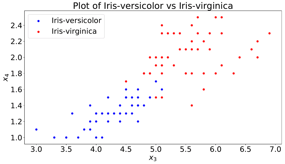
Scatter plot of petal length against petal width for Iris versicolor in blue and Iris virginica in red. The two clouds meet and interleave along a diagonal band around petal length 5 centimetres, with roughly half a dozen points of each class inside the other's territory. — Petal length ( $x_3$ ) against petal width ( $x_4$ ) for the hard pair, one of the 18 scatter plots `SVM/PlotClassesv2.py` wrote, report Fig. 21, p. 22. The overlap in the middle is the whole reason this pair tops out around 94.5% and the other two reach 100%. Load this pair into the playground above (it is a preset, with all six feature pairs selectable) and no value of C gets you a clean split.

The widget below is the report’s own numbers: mean test accuracy over 50 random 60/40 splits, for every one of the thirteen $C$ values, read out of SVM/OutputStats.npz. Table 5 in the report prints four of those thirteen columns; this is all of them, with the interquartile band across the 50 trials.

InteractiveThe report's Iris results, all thirteen values of C

Mean test accuracy, versicolor vs virginica, from `SVM/OutputStats.npz`.
C	Linear	Polynomial	Radial basis	Sigmoid
0.016	47.40	93.45	47.45	46.85
0.03	47.40	93.40	47.40	46.75
0.06	67.85	93.30	74.15	47.00
0.12	89.35	93.15	93.15	47.05
0.25	93.10	93.50	93.60	47.40
1.00	94.50	93.10	93.40	91.55
4.00	94.70	93.30	93.95	93.55
64.00	93.65	92.65	92.95	93.85

With JavaScript on, this is a chart of all thirteen C values for any of the three class pairs, with quartiles and a readout of the exact numbers.

Table 5 as the report prints it (p. 25), transcribed from SVM/Output/MeanTabel.tex:

Problem	C	Linear	Polynomial	Radial basis	Sigmoid
Versicolor vs Virginica	0.03	47.40	93.40	47.40	46.75
	0.25	93.10	93.50	93.60	47.40
	1.00	94.50	93.10	93.40	91.55
	64.00	93.65	92.65	92.95	93.85
Versicolor vs Setosa	0.03	85.35	99.80	77.75	53.35
	0.25	100.00	99.45	100.00	100.00
	1.00	100.00	99.50	100.00	100.00
	64.00	100.00	100.00	100.00	100.00
Virginica vs Setosa	0.03	92.95	99.30	78.40	53.05
	0.25	100.00	98.65	100.00	99.65
	1.00	100.00	99.05	100.00	100.00
	64.00	100.00	100.00	100.00	100.00

And Table 6 (p. 26), the parameters that got the lowest validation error, from SVM/Output/ParamsTabel.tex:

Problem	Kernel	d	γ	C₀	C
Versicolor vs Virginica	Linear	–	–	–	8.00
	Polynomial	2.00	1.18	40.91	0.06
	Radial basis	–	0.62	–	4.00
	Sigmoid	–	0.24	0.13	64.00
Versicolor vs Setosa	Linear	–	–	–	0.12
	Polynomial	2.00	0.25	0.02	4.00
	Radial basis	–	0.25	–	0.25
	Sigmoid	–	0.09	0.09	1.00
Virginica vs Setosa	Linear	–	–	–	0.12
	Polynomial	2.00	0.28	0.05	1.00
	Radial basis	–	0.25	–	0.25
	Sigmoid	–	0.09	0.09	1.00

Three things come out of those two tables.

The separable pairs are boring, and that is the finding. Once $C \ge 0.25$ , every kernel scores 100% on both setosa problems. The gap between setosa and everything else is wide enough that no point ever needs to fall inside the margin, so the extra capacity of a polynomial or radial basis kernel buys nothing, and the converged parameters in Table 6 agree, settling on small $\gamma$ and small $C_0$ , which is to say on the simplest function in the family.

The hard pair rewards a middle $C$ . Versicolor vs virginica peaks at 94.50% with a linear kernel at $C = 1$ in Table 5, and the full sweep (which the report does not print but the .npz does) peaks a little higher still, at 94.70% at $C = 4$ , before drifting back down to 93.65% at $C = 64$ . Too small and the boundary dissolves; too large and it contorts itself around individual overlapping points and generalises worse. The report says this in one sentence in §4.4 and it is the correct sentence.

Table 6’s $C$ values are not to be trusted, and the report says so. The selection rule takes the first $C$ reaching the highest validation score, and with only five resplits of a 60-point training set on those two problems there are ties everywhere. That is how the linear kernel ends up recorded at $C = 0.12$ on both setosa pairs when the full sweep is already at 100% mean test accuracy by $C = 0.06$ , and on the versicolor–setosa pair $C = 0.12$ is, on my own solver, the last value at which not one support vector is free of its bound. The report flags this itself in §4.4: “these C values are relatively small and may be sub-optimal”. More data, or more resplits, would break the ties.

What I would change

The sparsity argument holds up, and I still think it is the most interesting thing about the model, more interesting than the accuracies, which on Iris are a foregone conclusion. What I would change is around it.

The grid search is the weak part. Twelve rounds of coarse-to-fine, on three problems, four kernels and thirteen values of $C$ , across 50 trials, with a 40-process pool, is a lot of compute spent to distinguish 93.4% from 93.6% on 100 flowers, and a good chunk of it, as noted above, was spent refining parameters the linear kernel ignores. The honest version of this experiment is smaller: one coarse grid, and the compute saved spent on more trials so the error bars mean something.

I would also not evaluate a sigmoid kernel without saying what it is doing. It is in the table because LIBSVM offers it, not because there was a reason to think $\tanh$ of an inner product was a sensible similarity for flower measurements, and its results are the least interpretable in the set.

The thread this sits on is worth naming, though. The previous post built a Gaussian process, which is the other kernel method in the same assignment: it also writes predictions as a weighted sum of kernel evaluations against the training data, and it also never builds $\boldsymbol\phi$ explicitly. The difference is exactly the one this post is about. The GP keeps every training point in its predictive mean and pays $O(N^3)$ for the privilege; the SVM’s optimality conditions hand back a subset and let you throw the rest away. Kernel methods trade dimensions for data points, and the SVM is the one that then gives most of the data points back.