Blog · Regression ·
Overfitting, explained by fitting a sine wave ten different ways
Ten noisy points, polynomials of order 0 to 9, and a training error that falls to zero while the curve becomes useless, plus the reason least squares is not a heuristic at all.
- interactive
- regression
- overfitting
- maximum-likelihood
- numpy
The first assignment of the intelligent-systems module handed us ten numbers and asked us to find the function that made them. Ten numbers is not much. The whole point of the exercise, which I did not appreciate until I plotted the ninth-order fit, is that ten numbers is exactly enough to be lied to by your own error function. I wrote the results up as a report for the module, and most of the code, the figures and the quoted lines in this post come from that write-up.
Ten points and a polynomial
The setup is one input , one target , and pairs of them. I want the function that generated the targets, knowing that something noisy happened between and the I was given.
I fit a polynomial, and the report’s justification for that choice is the one I still give: most functions you care about are well approximated by the first few terms of their Taylor expansion, so a polynomial is a reasonable general-purpose guess when you have no reason to prefer anything else.
is the order, and it is the only knob that controls how complicated the model is allowed to be. Stack one per data point and you get the design matrix , which is .
In code that is a Vandermonde matrix built one row at a time:
def createSQM(x,M):
    vfunc = np.vectorize(lambda x,i: x**i)
    ilist=np.arange(M+1)
    xlist=np.repeat(x, M+1)
    return vfunc(xlist,ilist)

def getXMatrix(Xlist,M):
    out = np.empty((0,M+1))
    for x in Xlist:
        out = np.append(out,createSQM(x,M).reshape((1,M+1)),axis=0)

    return out
One detail that matters for reproducing anything: the dataset file contains only the
targets. The inputs are reconstructed as points evenly spaced on :
np.arange(0, 1+1.0/len(t), 1.0/(len(t)-1.0)). The widget below does the same thing.
Least squares, in closed form
Minimise the sum of squared residuals:
Differentiate with respect to , set the gradient to zero,
and you land on the normal equations:
No iteration, no learning rate, no epochs. The entire fitting procedure is three lines:
def Error(W,x,t):
    return 0.5*np.sum(np.square(np.dot(x,W)-t))

def getLogLiErr(W,x,t,Beta):
    return 0.5*Beta*np.sum(np.square(np.dot(x,W)-t))+0.5*len(t)*np.log(Beta/(2.0*np.pi))

def getOptimalW(x,t):
    return np.linalg.solve(np.dot(x.T,x),np.dot(x.T,t))
getOptimalW forms the Gram matrix
explicitly and hands it to np.linalg.solve, which is an LU factorisation with partial
pivoting, not pinv, not a QR least-squares solve, and with no regularisation term
anywhere. That choice comes back to bite later in this post.
Maximum likelihood gives the identical answer
Now do it properly. Assume the target at each input is the model output plus Gaussian noise of precision :
Take the log:
The only term that depends on is the last one, and it is times the least-squares error. Maximising the likelihood over is therefore exactly minimising : same normal equations, same weights, same curve.
This is the sentence I would put on the wall of every introductory course. Least squares is not a sensible-looking heuristic that people happen to use. It is the maximum likelihood estimator for a linear model with independent Gaussian noise of constant variance. Every time you reach for it you are asserting that noise model, whether or not you say so out loud. If your noise is heavy-tailed or heteroscedastic, least squares is not “still a reasonable choice”, it is the right answer to a question you did not mean to ask.
The report plots both, side by side, for order 4. They are the same plot, and that is the entire point of the figure:
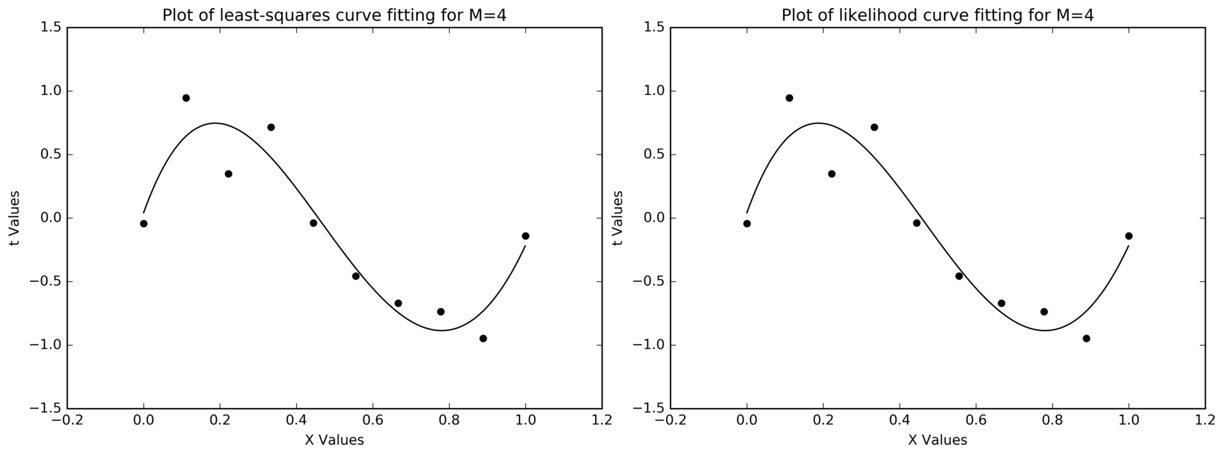
Least squares (left) and maximum likelihood (right) at , produced by two separate code paths that land on identical curves.
Crank it to nine
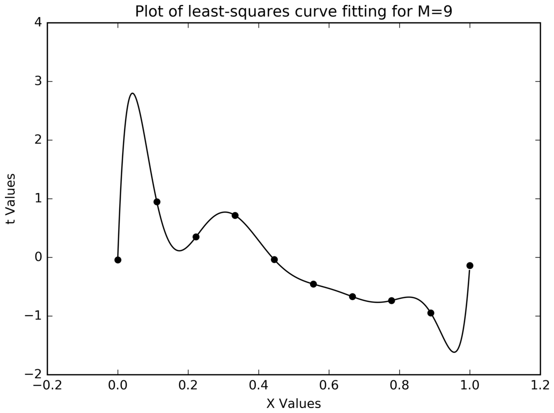
Ten data points. An order-9 polynomial has ten coefficients. From the report:
The data has 10 degrees of freedom, all of which can be accounted for by the parametric equation. Due to this, the best fit for the data is one that goes through all the points. This has a very low error function but often does not generalise well to new data.
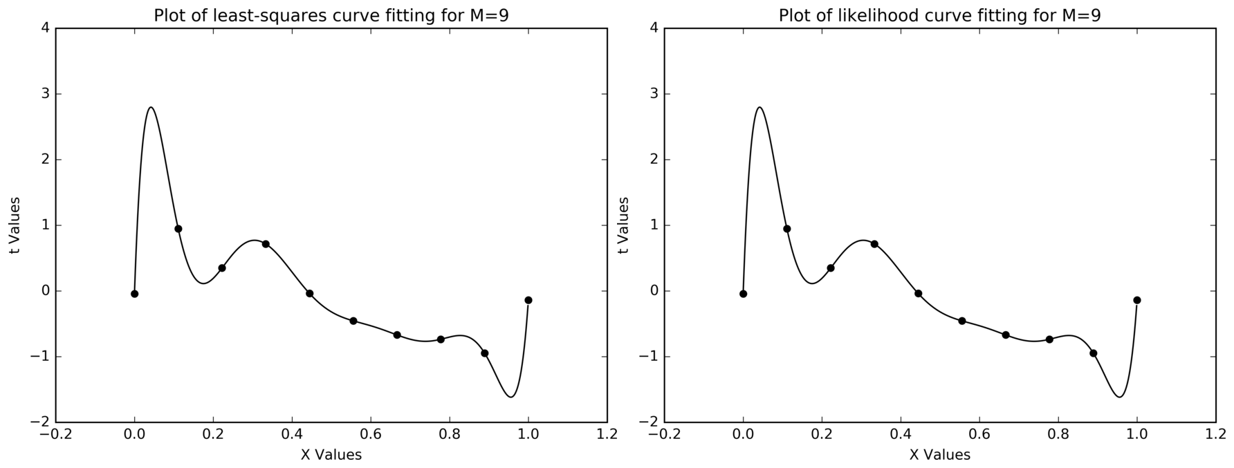
. The curve interpolates all ten points perfectly and is worthless everywhere between them.
The curve passes through every point and, in doing so, spikes to just past the left edge of the data and dives to near the right. Recomputing the fit, the largest coefficient at is about ; at it is . Huge opposing coefficients cancelling each other to five significant figures is the numerical signature of this failure, and it is why the ninth-order Gram matrix is nearly singular.
Meanwhile the training error does what training error always does:
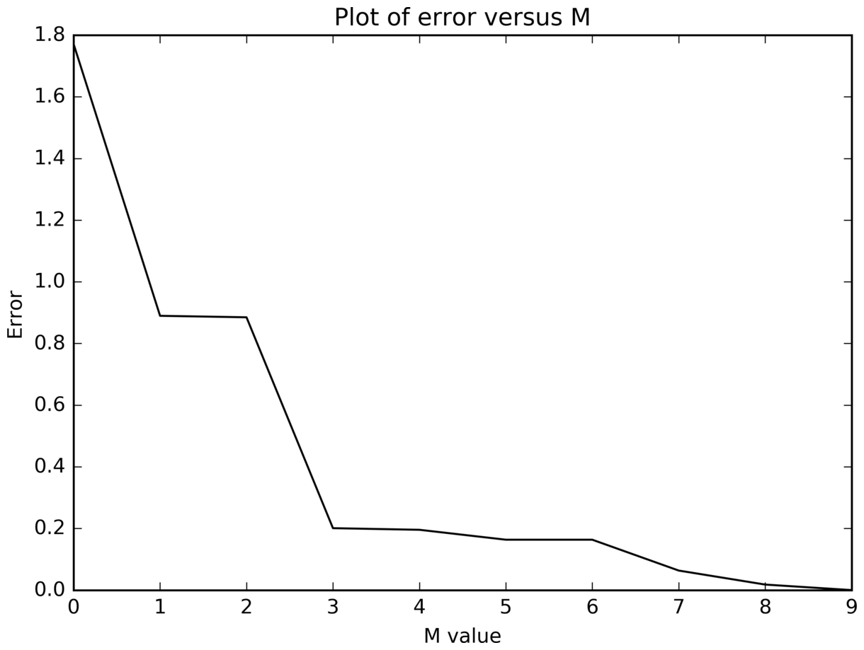
against .
| RMS residual | ||
|---|---|---|
| 0 | 1.771 | 0.595 |
| 1 | 0.890 | 0.422 |
| 2 | 0.885 | 0.421 |
| 3 | 0.201 | 0.200 |
| 4 | 0.196 | 0.198 |
| 5 | 0.163 | 0.181 |
| 6 | 0.163 | 0.181 |
| 7 | 0.063 | 0.113 |
| 8 | 0.018 | 0.060 |
| 9 |
The plateaus are the interesting bit. Nothing happens between and , and nothing happens between and , because the underlying function is odd: has no even-order terms, so the even coefficients have almost nothing to explain. Adding one buys you essentially nothing. The report makes this argument later, to justify why the Bayesian evidence peaks at ; it is already visible here, in a plot that is otherwise just a monotone slide toward zero.
And monotone is the problem. can never increase with , because the order- model space is contained in the order- one: the larger model can always set the new coefficient to zero and match. A quantity that cannot go up is not a model-selection criterion. It is a measurement of how much freedom you gave the model.
The sting: does not survive the argmax
Go back to the log-likelihood. The precision is right there in the expression, and it drops out of the maximisation over completely, it multiplies a term whose minimiser it cannot move. So maximum likelihood over the weights hands you a curve and tells you nothing whatsoever about how much to trust it. You have to supply yourself, and here it was simply asserted: the report assumes the data was generated with (a noise standard deviation of about ).
You can see the consequence in the repo’s second error plot. getLogLiErr is called with
and its output is plotted against :
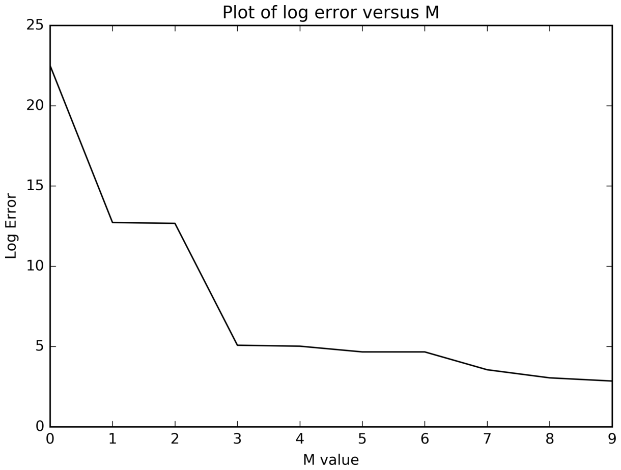
The log-likelihood error against . Same shape, different axis.
It is the same curve. Look at the function again: it returns , which for fixed and is multiplied by and shifted by . It cannot distinguish anything the first plot could not. That was the real lesson of the whole exercise: I had computed a likelihood, felt like I had done something more principled than curve fitting, and produced a rescaled copy of the plot I already had.
Do it yourself
Everything above is one solve of a small linear system, so it runs comfortably in the browser at pointer speed. Click on the plot to add a point, drag one to move it, shift-click to delete it. The slider is .
The moment worth chasing: set to 9, then add an eleventh point anywhere. Eleven points, ten parameters: the curve stops interpolating, jumps off zero, and the sparkline’s right-hand end lifts off the floor. Nothing about the model changed. Only the arithmetic of degrees of freedom did.
With JavaScript on, this becomes a canvas you can click to place points, with a slider for the polynomial order, live readouts of E(w) and the log-likelihood error, and a log-scale sparkline of error against M.
The second preset is the repo’s other dataset: 80 samples, used later in the report for Bayesian model comparison. Load it and the picture inverts: with eighty points there is nothing for a ninth-order polynomial to interpolate, the error-vs-M sparkline flattens out after , and every order from three upward draws more or less the same sine. Overfitting is not a property of the model. It is a property of the ratio.
The widget is a direct port of the original fitting script, with one deliberate
departure. NumPy’s np.linalg.solve on a ninth-order Gram matrix built from arbitrary
user-placed points will happily return garbage or blow up, so the widget factorises with
Cholesky and adds an escalating ridge to the diagonal until the factorisation succeeds,
then reports the ridge it needed. Drag two points close together at and you can
watch it kick in. The original script never had to deal with this because its ten inputs
were always evenly spaced; that is not a virtue of the code, just of the data.
Why there is no WASM here
Several posts in this series push work into Rust compiled to WebAssembly because the alternative is a page that stutters. This is not one of them, and it is worth being explicit about where the line falls. The heaviest thing this widget does is form a Gram matrix and Cholesky-factorise it, a few thousand floating-point operations, ten times over for the sweep across all orders, on every pointer move. That is microseconds. Reaching for WASM here would buy nothing measurable and cost a build step, a fetch and a memory boundary. The interesting engineering question is never “is this fast in principle”, it is “is this the part that is slow”.
Next
Least squares gave a point estimate of and no error bars, and fell out of the maths without leaving a trace. The next post puts a prior on the weights instead and gets a predictive variance out of the same ten points, including error bars that fan out where the data is missing, which is the single most persuasive figure in this repo. That is the Bayesian treatment, and it is where the overfitting problem starts to solve itself.