Blog · Regression ·
Error bars for free: Bayesian linear regression and the evidence
A prior on the weights buys three things least squares cannot give you: a band that widens where the data is missing, immunity to the order-9 catastrophe, and a number that ranks models on training data alone.
- interactive
- regression
- bayesian
- model-selection
- evidence
- numpy
The previous post ended with a complaint. Least squares hands you a curve and nothing else: no sense of where it is guessing, and a training error that slides monotonically to zero while the curve becomes useless. The noise precision appeared in the likelihood and then dropped straight out of the argmax, so the machinery could not even tell you how wrong to expect it to be.
The fix in the same assignment was one change: stop asking for the best and ask for the distribution over . Three things fall out of that, and none of them cost anything beyond a second linear solve.
A prior on the weights
Same model as before: with , and the same design matrix stacked one row per data point. What changes is that gets a prior: a zero-mean Gaussian with a single precision shared across every coefficient, .
A Gaussian prior and a Gaussian likelihood give a Gaussian posterior, in closed form. Bishop 3.50 and 3.51, with the general , specialised to a zero-mean isotropic prior:
That is the whole fitting procedure. Four lines of code:
Sninv=alpha*np.eye(sudoM)+beta*np.dot(xMat.T,xMat)

MnEqns=beta*np.dot(xMat.T,tlist)

Mn=np.linalg.solve(Sninv,MnEqns)
...
Sn=np.linalg.inv(Sninv)
Compare that with the normal equations from the last post, . The only difference in the matrix being solved is on the diagonal. Bayesian linear regression with an isotropic Gaussian prior is ridge regression; the difference is that here the ridge parameter arrived as a statement about what you believe, and it comes with a covariance attached.
That covariance is the thing worth having.
The predictive variance, and why it is two terms
Ask the model for a prediction at a new input and you do not get a number, you get a Gaussian. Its variance is
Read the two terms separately, because they mean completely different things.
The first, , is the noise on the observation. It does not depend on , it does not depend on the data, and no amount of extra data will shrink it. With it is a standard deviation of , and that is the floor: the band around any prediction can never be tighter than that.
The second term is the part that is actually informative. It is a quadratic form in , so it depends on where you ask. Ask somewhere the data pinned the weights down and it is small. Ask somewhere the data says nothing about, off the end of the range or in a hole in the middle, and has a large component along a direction of that the likelihood never constrained, and it grows. This is uncertainty about the function, not about the measurement, and it is exactly the quantity that least squares throws away.
The loop that evaluates it:
sigmaxlist=[]
for xp in xFineList:
    phi=createSQM(xp,sudoM).reshape((-1,1))
    sigma_2n=1/beta+np.dot(phi.T,np.dot(Sn,phi))
    sigmaxlist+=[np.sqrt(sigma_2n[0,0])]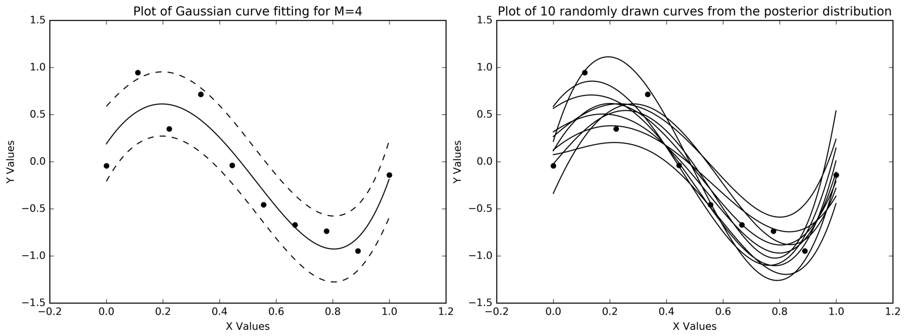
on the ten points. Left: the posterior mean with dashed lines at . Right: ten weight vectors drawn from , each plotted as a curve.
The right-hand panel is the same posterior seen from the other side. Rather than summarising it as a mean and a width, draw ten weight vectors from and plot the polynomial each one defines. Every curve there is a function the data considers plausible. Where they bunch together the model is confident; where they fan apart it is not. The two panels are the same information, and the sampled one is much harder to misread as “the answer, plus a bit of noise”.
Drawing those samples is the only part of this that is not a linear solve.
np.random.multivariate_normal does the work in the original; the widget at the bottom
of this page factorises and takes
with
standard normal, which needs one back-substitution and no matrix inverse at all.
Order 9 stops being a catastrophe
Here is the first thing that surprised me at the time. Fit the same ten points with (the order that in the last post drove a curve through every single point and spiked to off the left edge) and the Bayesian answer barely moves.
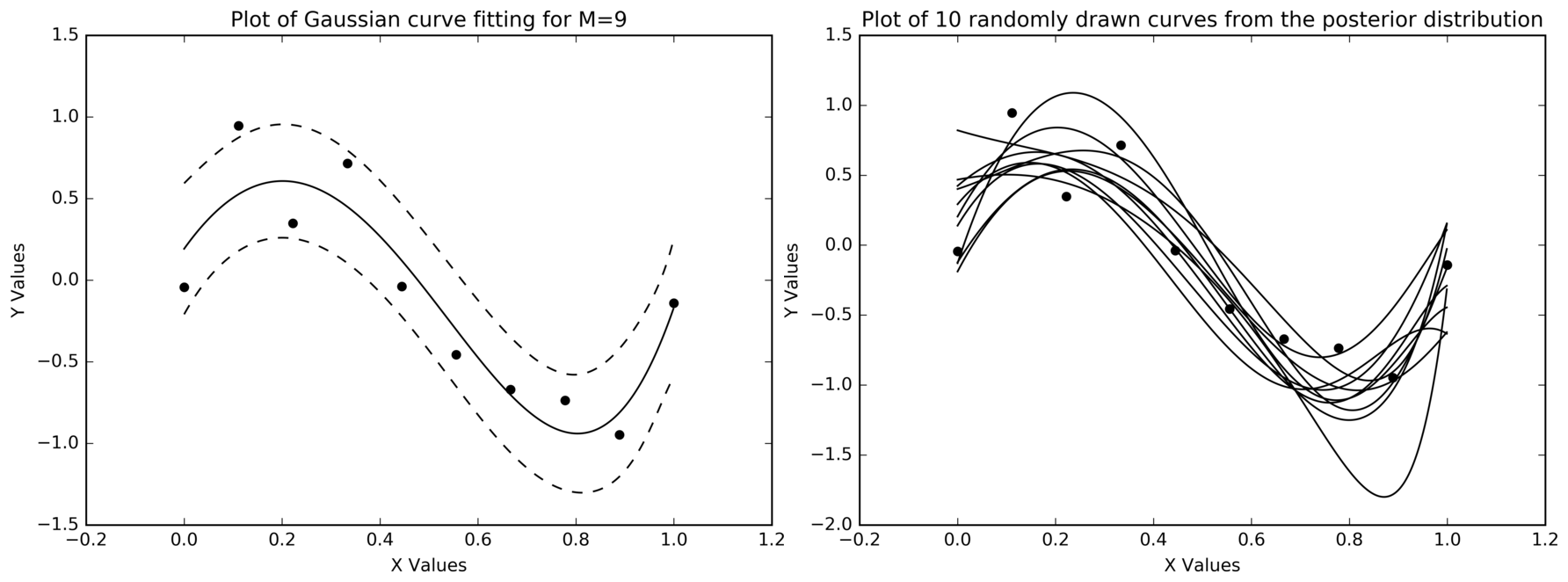
on the same ten points. Set this beside the previous figure: you have to look hard to find a difference.
The numbers, recomputed:
| least-squares | 29.2 | |
| Bayesian | 11.9 | 10.8 |
| posterior mean at | 0.190 | 0.192 |
| 0.398 | 0.401 |
Least squares at order 9 needs coefficients of order cancelling each other to five significant figures. The posterior mean needs nothing bigger than , a smaller largest coefficient than the order-4 fit uses. The report explains why by pointing at Bishop 3.55, the log posterior over the weights, whose weight-dependent part is
and then, in the report’s words:
From the term , it is possible to see that is negatively influenced by adding more parameters. Due to this, the Bayesian regression function will limit its effective complexity to keep the effects of this term low.
That is the right intuition, but it is worth being precise about what it does and does not say, because “adding a parameter is penalised” is not quite it. Adding a coefficient that is genuinely zero costs nothing. What the term forbids is the specific pathology of the last post: two enormous coefficients that cancel. Those cost times the sum of their squares, and of penalty buys you an improvement in fit of, at best, the last few decimal places of the residual. The posterior simply never goes there. Order 9 has ten parameters available and quietly declines to use most of them.
Delete five points and watch the band open
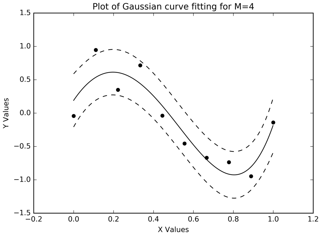
This is the figure that sold me on the whole approach, and it is the one I would keep if I could keep only one thing from this repo. Take the same ten points, delete five of them from near the start (indices 1 through 5, which the script simply comments out), and refit at .
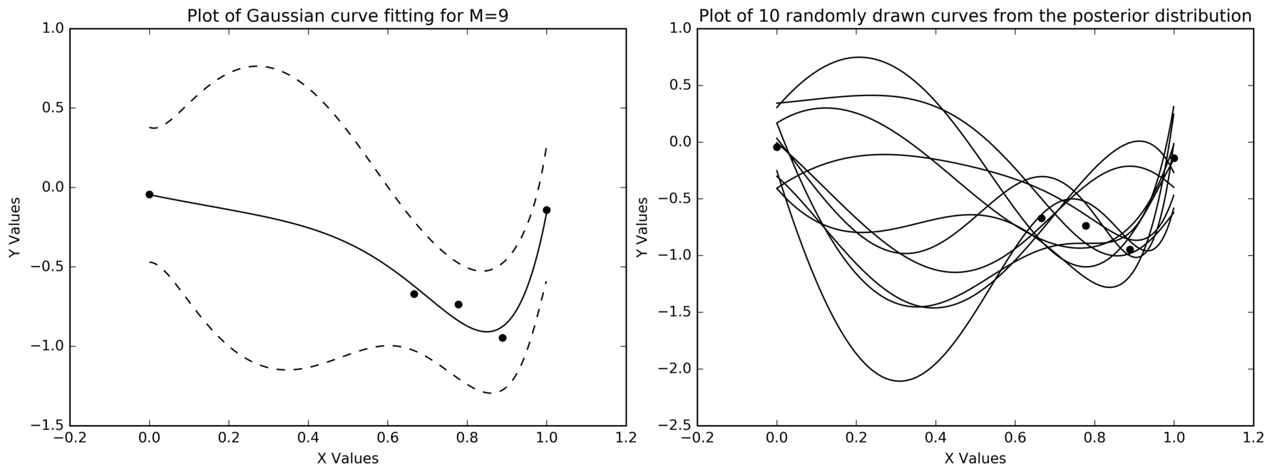
The same model, five points removed. The band fans open exactly over the hole and closes again where the surviving points are.
The report’s own comment on this is the most useful sentence in it:
This result is very useful for real life applications, where the certainty of the predictions is required to make an informed decision.
Which is understated. The mean curve through that gap is a smooth, confident-looking, entirely fabricated interpolation. Every method in the last post would have drawn it and said nothing. This one draws it and hands you the caveat in the same object, and the right-hand panel (ten sampled functions swinging between and across the hole) makes it impossible to pretend otherwise.
The evidence: ranking models with no held-out data
Everything so far treats as given. The last post established that training error cannot choose it, because training error cannot increase with . Cross-validation can choose it, at the cost of throwing away data and refitting many times. There is a third option that costs one extra determinant.
If indexes the candidate models, Bayes’ rule gives , and with a uniform prior over the ten orders the posterior over models is just the normalised evidence , the probability of the data under the model with the weights integrated out:
That is Bishop 3.78. The integrand is a Gaussian, so the integral is available in closed form (3.85):
with
Note that is the same matrix as : you already factorised it to get the posterior mean. The from 3.85 cancels the from 3.78 exactly, which is why the log evidence collapses to Bishop 3.86:
One line, with sudoM being the number of basis functions
and A the matrix already built for the posterior:
p_DGM=((sudoM*np.log(alpha)+N*np.log(beta)-np.log(np.linalg.det(A))-N*np.log(2*np.pi))/2.0)-E_MnThe term that does the work is . Each extra basis function adds a row and a column to , multiplying its determinant by roughly the curvature of the posterior in that new direction, and the evidence pays for it. A model that is more flexible than the data warrants wins on and loses more on . Nothing was held out, nothing was refitted; Occam’s razor arrives as a determinant.
Running it on eighty points
The evidence sweep uses the second dataset: eighty targets generated the same way as the first ten. Here is the whole sweep, recomputed from that dataset with the same and :
| behind the best (nats) | ||||
|---|---|---|---|---|
| 0 | −246.24 | −207.8 | 262.95 | |
| 1 | −106.61 | −68.1 | 118.51 | |
| 2 | −109.02 | −70.5 | 117.45 | |
| 3 | −38.47 | best | 22.7 % | 44.77 |
| 4 | −38.61 | −0.14 | 19.7 % | 43.71 |
| 5 | −39.30 | −0.83 | 9.9 % | 43.40 |
| 6 | −39.24 | −0.77 | 10.6 % | 42.52 |
| 7 | −39.06 | −0.59 | 12.5 % | 41.66 |
| 8 | −39.03 | −0.56 | 13.0 % | 41.01 |
| 9 | −39.14 | −0.67 | 11.6 % | 40.58 |
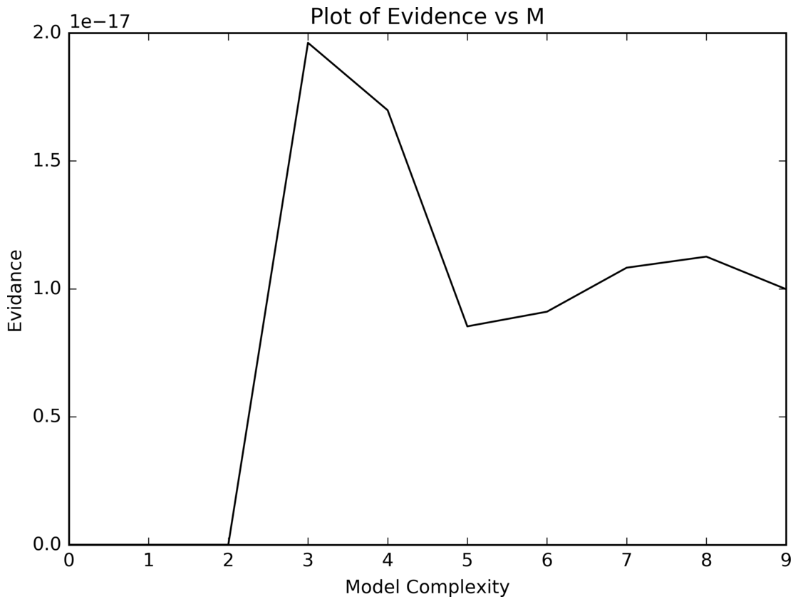
The report’s plot. The axis is linear and in units of ; the peak sits just under at , which is the in the table above. My port reproduces every point on this curve.
wins, and the report’s explanation of why is the nicest observation in the whole write-up. The data came from a sine, and
is odd, so the even powers of contribute nothing, and the factorials in the denominators kill the higher terms fast. A cubic is the smallest polynomial that has both the terms a sine actually needs.
That argument is easier to see in the log column than in the plot. The plot’s linear axis makes look like zero, which flattens the most interesting part of the story:
- : adding the linear term is worth 140 nats, a factor of . The first Taylor term.
- : adding makes the evidence go down, by 2.4 nats. A bigger, strictly more flexible model that the data likes less: the even-power term earns nothing and still has to pay for its own determinant. That single negative step is the oddness of the sine showing up directly in the arithmetic.
- : adding is worth 70 nats. The second Taylor term.
- : down again, by 0.14 nats. Another even power, another small loss.
- Past the whole thing is flat to within a third of a nat. Those differences are not meaningful, and I would not read the small rise at as anything at all.
So the reading is not “the evidence picks ” but “the evidence picks odd orders, strongly prefers 3, and cannot distinguish 5 through 9 from each other”. Even the winner only takes 22.7 % of the posterior mass over models. That matters for the next section.
Averaging instead of choosing
If the evidence says is only 22.7 % likely, why commit to it? Bishop 3.67 says you do not have to: predict with a mixture of all ten models weighted by . The mean and variance of that mixture come from Trailovic and Pao:
The second one is worth reading twice. The mixture’s variance is the average of the component variances plus the spread of the component means: disagreement between models is itself uncertainty. Nine lines:
Ap_DGMlist=Ap_DGMlist/np.sum(Ap_DGMlist)
FCombined=np.dot(Ap_DGMlist,predictorList)

sigma2=0
for mui,sigmai,w in zip(predictorList,sigmaxlist,Ap_DGMlist):
    sigma2+=w*((mui-FCombined)**2+sigmai)

sigma=np.sqrt(sigma2)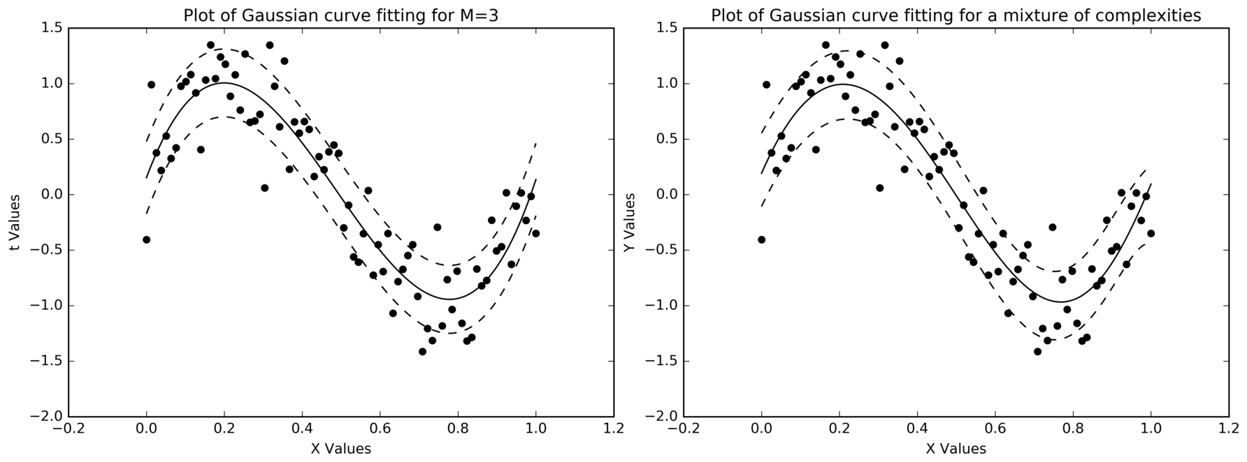
Left: the winning single model, . Right: the evidence-weighted mixture over all ten.
The report’s conclusion is that you may as well use the most probable model, since the mixture costs ten fits and buys you almost nothing, and on this data that is plainly right. It is worth saying why it is right here and would not be everywhere: the ten models are nested and their means agree almost everywhere, so the disagreement term is tiny. Average over ten genuinely different model families and it would not be.
The coda that was never coded
Every number above assumed and . The report’s last section describes how to stop assuming them: maximise the evidence with respect to the hyperparameters too. Compute at the current guess, then
and re-estimate with Bishop 3.98 and 3.99,
iterating to convergence: the whole thing is a fixed-point loop over two scalars.
Do it yourself
The widget below is a port of the posterior-fitting script and the corrected evidence script together. Click the plot to add points, drag to move them, shift-click to delete one. The sliders are , and ; they start at the report’s values.
Three things to try, in order of how much they taught me:
- Gouge a hole. Press gouge a gap and drag across a stretch of the plot. The points in that stretch are deleted and the band balloons over the gap: the report’s figure, but with the hole wherever you want it, and the readout tells you how many times the noise floor has reached.
- Let the evidence choose. Tick let the evidence pick M. It lands on on both of the repo’s datasets, with 22.7 % of the model posterior on the eighty points and 35.6 % on the ten. Then press the report’s gap, which deletes the same five points as the figure above: with only the endpoint and a cluster near left, the evidence collapses onto with 87.8 % and refuses to fit anything at all. Nothing is held out at any stage.
- Turn down. At , drag from down to and
watch the prior let go:
max |mₙ|in the readout climbs from to , and the posterior mean starts to grow the spikes of the least-squares fit from the last post (, and worse between the points). That single slider is the whole difference between the two posts. It has to go a long way down before anything visible happens, which is itself the point: a prior variance of per coefficient is barely an opinion, and it is still enough.
With JavaScript on, this becomes a canvas you can click to place points, with sliders for the polynomial order and the two precisions, a toggle between the ±σ band and ten functions sampled from the posterior, a brush that deletes a whole region so you can watch the band open over the gap, and a live bar chart of p(M|D) across orders 0 to 9.
The bar chart under the plot is the evidence, normalised over the ten orders, recomputed for whatever points are on the canvas. The grey number under each bar is how many natural logs behind the winner that order is, because a bar that rounds to zero on a linear axis can be two hundred logs behind, and the difference between “slightly worse” and "" is not one a bar chart can draw.
Under paste your own data, or export the fit you can drop in your own numbers: one
x, t pair per line, or a single column of targets in the shape both of the repo’s
dataset files are in, which get spread evenly over the way the scripts do it. The
CSV export gives you the mean and the band on a fine grid; the JSON export gives you
, the full covariance , and the log evidence of all ten
models.
One small pleasure of implementing this: the order-9 solve needed no numerical babysitting at all. The last post’s widget had to add an escalating ridge to the diagonal because goes singular on user-placed points. Here is positive definite for any , so the Cholesky always exists and the escalating ridge is already there, by name, with a probabilistic interpretation. The prior fixes the linear algebra as a side effect of fixing the statistics.
What is still wrong with this
Two things, and the second one is the subject of the next chapter.
The first is that and were asserted rather than learned, and the section that would have learned them was never written as code.
The second is bigger. Everything here is exact and closed-form because the model is linear in , and that required me to pick up front. I chose monomials, and then spent an entire section using the evidence to decide how many of them to use. But the evidence can only rank the models I thought to write down. It has nothing to say about whether polynomials were the right basis in the first place, and on data that was not generated by something with a nice Taylor series, they are not.
The obvious next question is whether you can avoid choosing a basis at all: put the prior directly on the function instead of on the coefficients of an expansion of it. You can, by marginalising away and keeping only inner products between data points, and what comes out is a Gaussian process. That is the next repo, from assignment 3 of the same module two months later, and it opens by doing exactly this derivation in reverse.