Blog · Bayesian filtering ·
How many particles, and how wrong can your first guess be?
Closing the Bayesian-filtering arc with the two questions every particle-filter engineer actually asks, answered by Monte-Carloing them live in the browser: Rust and WASM in a Web Worker, sweeping tens of millions of particle-updates behind a progress bar.
- interactive
- particle-filter
- extended-kalman-filter
- monte-carlo
- rust
- webassembly
- bayesian-filtering
Three posts ago I derived the Kalman filter from a voltmeter. Two posts ago its extended cousin locked onto the wrong range and stayed there. Last post a cloud of four thousand weighted guesses held two stories at once (close-and-slow, far-and-fast) for exactly as long as the lighthouse’s one bearing gave it no reason to pick. That is the whole arc: 1-D → nonlinear → multi-modal, each post breaking the previous one’s assumption. This one closes it by asking the two questions nobody answers with a derivation: how many particles is enough, and how wrong can the first guess be before it matters. §5.5–5.7 and §6.5–6.7 of the report (Experiments 5, 6 and 7) answer both, with a third experiment thrown in that answers a question I didn’t expect: what happens to the multi-modality itself when you add a second kind of measurement.
The code for this post is drawn from three of the report’s experiment scripts
(and their loaders), the problem definition Dataset C uses, and two more
functions from the shared utilities module. The widget itself is new work,
not a port of an experiment script: a Rust crate, pf-wasm, compiled to
WebAssembly and run in a Web Worker, because “run the sweep live” costs tens
of millions of particle-updates: the one place in this four-post arc where
that toolchain earns its keep rather than being a distraction.
Question one: how many particles?
§5.6 sweeps : the report says “from to using steps
of 100”; the script that actually produced the figure loops
range(200, 10200, 200), 50 points from 200 to 10000. Small discrepancy, but
worth noting since I’m about to lean on the code, not the prose, for the
widget’s own point count. Everything else is fixed at dataset
B’s usual values (the same , , as post
19) except the initial guess, which here is the
near cluster, not the true start:
initP = np.array([[0.5**2,       0,      0,       0],
                  [0     , 0.005**2,      0,       0],
                  [0     ,        0, 0.3**2,       0],
                  [0     ,        0,      0, 0.01**2]])
initX = [0.0, 0.0, 0.4, -0.05]
...
runs = 20
def evaluateAllFiltersPartial(numberOfParticals, currX):
    return evaluatePFFilterLessMemory(problem, numSamples, X0Real, numberOfParticals, K,
                               R, Q, initP, initX, [0,1,2,3])
The driving loop, trimmed. evaluatePFFilterLessMemory only ever builds one
filter, ParticleFilterSIRWithJitter (SIR, always resampling, jitter on) and
runs it 20 times per . Fig. 12, page 22:
The report’s own advice, §7 p.24, is the whole reason this post has a live sweep instead of a screenshot of one: picking by “however many the CPU can afford” wastes resources, and picking it from a general rule of thumb gets the wrong answer for your , and dimensionality. The right move is to run the algorithm a few times at increasing , plot error against , and read the knee off the curve. So: press play below rather than read mine off a report page.
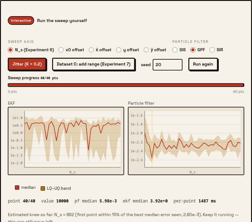
With JavaScript on, this Monte-Carlos the sweep itself in a Web Worker: pick the axis (particle count, or the initial guess’s offset along one of the four state components), pick SIS, GPF or SIR, toggle jitter and Experiment 7’s range measurement, and press Run. Median and interquartile-range bands fill in left to right as each point finishes; a Stop button is always live.
I ran it myself at from 100 to 10000 (GPF with jitter, 20 runs a point,
matching that script’s own runs = 20): the median MSE drops from about
at to – by and
stays in that band out to 10000, the same decaying-then-flat shape as Fig.
12, noisier because 20 runs a point is what the report itself budgeted, not
because the widget cut corners. The knee marker (dashed, “smallest
within 15% of the best seen”) lands around 1000–2000 in my runs, a little
earlier than the report’s “sufficient by 4000”, both are reading noise off
the same shape, and that is rather the point: your curve, for your problem,
is the one to trust, and this one visibly moves as more points stream in.
Question two: how wrong can the first guess be?
§5.5 asks the complementary question: fix , and instead push the initial estimate away from the truth:
X0Real = np.array([-0.05, 0.001, 0.7, -0.055])
weightings = [-15.0, 8.0, 15.0, -8.0]
...
def evaluateAllFiltersPartial(initX, currX):
    initP = np.eye(4)*(1e-6+(X0Real-initX)**2)
    return evaluateImportantAllFiltersLessMemory(problem, numSamples, X0Real, numberOfParticals, K,
                               R, Q, initP, initX, [0,1,2,3])
...
for axis in range(4):
    for percentageOfActual in np.linspace(0,1,100):
        X0RealValue = X0Real.copy()
        X0RealValue[axis] += weightings[axis]*percentageOfActual
Read that carefully, because it is a nice piece of engineering: the true
start X0Real never moves: only the guess X0RealValue walks away from it,
one state axis at a time, up to in position or in velocity. And
the guess’s own uncertainty, initP, grows to match: . The
filter is told, correctly, “I might be off by this much”, which for a
particle cloud means the true state sits about one standard deviation from
the sampled mean at every point on the sweep, always recoverable in
principle. Whether it is recovered in practice is the experiment.
Figs. 10 and 11, page 21, split the two filters onto separate charts, because their axes don’t share a scale: the EKF’s climbs to – while the PF’s stays at –, four to ten orders of magnitude apart. My own re-run (widget defaults, GPF with jitter, , 50 runs a point: my own budget for a browser sweep, half the report’s and a twentieth of its 1000 runs) lands on the same shape and very nearly the same scale:
| Axis (offset at full throw) | EKF MSE at offset 0 | EKF MSE at full offset | PF MSE at full offset |
|---|---|---|---|
| (, ) | |||
| (, ) | see below | ||
| (, ) | |||
| (, ) |
The particle filter earns its reputation on three of those four columns, barely moving while the EKF detonates. The fourth, , is the exception, and it is worth showing rather than hiding.
Why: the report’s own explanation
§7’s closing paragraphs, rephrased: the further the initial guess sits from the truth, the faster the true object would have to be moving to produce the same sequence of bearings, so distance from the guess, along a velocity axis especially, doesn’t just add error, it manufactures alternative stories for the data to tell. That is literally the source of the bimodality post 19 built its whole argument on; Experiment 5 is the same phenomenon shown as a dial rather than a snapshot. And the flip side, worth remembering before the next section: an object that is close and moving fast has few alternative explanations: it’s already near the edge of what the sensor can distinguish, so the EKF does comparatively better the closer and faster the target is. Distance from truth is what buys the particle filter its advantage, not multi-modality as some intrinsic property of bearings-only tracking.
Question three (a bonus): what if you add a range measurement?
Experiment 7 changes the problem, not the initial guess. Dataset C’s problem definition keeps the bearing but adds a second measurement, the squared range:
class TestProblem4(ProblemType):
    def __init__(self, r=0.005**2, q=0.001**2):
        self.n,self.m = 4,2
        ...
    def h(self, x,k):
        return np.array([np.nan_to_num(np.arctan2(x[2],x[0]))
        ,x[2]**2+x[0]**2])
    ...
    def Jh(self, x,k):
        x2py2=np.nan_to_num(1.0/(x[0]**2+x[2]**2))
        return np.array([[-x[2]*x2py2, 0, x[0]*x2py2, 0],
                         [2*x[0], 0, 2*x[2], 0]])
Squared range, not range, which is why the Jacobian’s second row is the clean rather than needing a square root anywhere. Experiment 7’s script sets , keeps , and runs all eight algorithms 1000 times. Table 3, page 22:
| Algorithm | EKF | IEKF | SIS | SISwJ | GPF | GPFwJ | SIR | SIRwJ |
|---|---|---|---|---|---|---|---|---|
| Mean “RMSE” () | 5.43 | 0.31 | 0.89 | 1.38 | 0.14 | 0.23 | 0.16 | 0.44 |
The point isn’t the table, though: it’s what happened to the EKF compared with dataset B. Bearing-only, its mean MSE on this same starting point is (my re-run; the report’s own dataset-B baseline, §6.3, is , see post 19). Add the range measurement and it drops to , better than a thousand-fold. The particle filter improves too (mean MSE roughly in my re-run, about ), but nowhere near as dramatically, because it didn’t need saving in the first place. The moral I take from it, and now believe: it is not that particle filters beat Kalman filters. It’s that a Gaussian can’t describe a multi-modal posterior, and a range measurement is one way to stop the posterior being multi-modal at all. Once it isn’t, the EKF is not just “usable again”: it goes back to being the better tool, because it is cheaper.
Why: cost
§7’s last real paragraph, rephrased, because it is the sentence I’d underline if I were reading this report cold: on a simple posterior, use the Kalman filter, because it is faster: its most expensive step is one matrix inversion (or a closed form, for small state dimensions), while a particle filter’s cost is times the per-particle work, run for every one of those particles. The saving grace is that per-particle work is embarrassingly parallel (a GPU or a many-core machine amortises it in a way a single matrix inversion cannot be split) and that particle filters spend their computation where the posterior actually has mass, which for a genuinely multi-modal problem, no fixed Gaussian ever can.
The crate: pf-wasm
The sweep above is real Monte Carlo, not a stored table: pick a point on an
axis, and the browser draws 20–50 independent noisy datasets, runs an EKF and
a full particle-filter cloud over 24 steps each, and repeats it across up to
40 points. At the top of that range (the offset sweep at , 50 runs,
40 points) that’s on the order of particle-state touches, not counting the per-particle
weighing and resampling passes. Plain JS handles this fine at post 19’s scale
(a few thousand particles at 60 fps); asked to do it 40 times over inside a
progress bar, it is the difference between “a few seconds” and “the better
part of a minute”, which is exactly the gap the pf-wasm crate exists to
narrow.
The crate is self-contained (calib-wasm is the camera-calibration crate,
gp-wasm the Gaussian-process one, nothing existing fit), follows
example-wasm’s C-ABI convention (wasm_alloc/wasm_free verbatim,
crate-type = ["cdylib"]), and has no dependencies, matching every other
crate in this workspace: a PRNG module (a bit-exact Rust port of the site’s
own seeded PRNG, sfc32 through splitmix32, verified against five next() and
five normal() values recorded from the TypeScript class at seed 42), a
model module (dataset B and C, matching the report’s own problem
definitions), an EKF module (the report’s own extended Kalman filter, ported
faithfully, including a bug I found while doing it, below), a particle-filter
module (the report’s SIS/GPF/SIR variants, log-domain weights, systematic
resampling and the corrected jitter formula post 19 already established),
and a sweep module, which runs one point of the chart and reports
mean/median/LQ/UQ for both filters. One exported function, sweep_point,
does the whole inner loop per call so a Web Worker can call it once per
sweep point and postMessage the result, which is how the chart streams in.
cargo test -p pf-wasm has seven cases, chosen to catch exactly the classes
of bug the sibling posts have found in this codebase: the PRNG matches the
TypeScript class bit-for-bit at a known seed, not just itself across two
instances; systematic resampling preserves the particle count and
concentrates on a single heavy particle (I rig one particle to hold nearly
all the weight and check it survives resampling at better than 90%);
log-sum-exp agrees with the naive computation on well-scaled values and stays
finite where the naive one underflows to zero (the whole reason scaleLogW
exists, see post 19); and a full sweep point is
bit-for-bit deterministic given a seed, run twice.
#[test]
fn log_sum_exp_matches_naive_when_naive_would_underflow() {
    let mut logw: Vec<f64> = vec![-800.0, -800.5, -799.2, -805.0];
    let naive: Vec<f64> = logw.iter().map(|v| v.exp()).collect();
    assert!(naive.iter().all(|&v| v == 0.0), "test setup: these should underflow");
    scale_log_w(&mut logw);
    let sum: f64 = logw.iter().map(|v| v.exp()).sum();
    assert!((sum - 1.0).abs() < 1e-9, "normalised weights should sum to 1, got {sum}");
}
From the particle-filter module’s test suite, trimmed. All seven tests pass.
Performance, measured rather than assumed
pnpm build:wasm pf-wasm produces a 40.9 kB binary, comfortably inside
the workspace’s ~200 kB-per-crate guideline, and about as small as a crate
with a PRNG, a 4-D EKF and a full particle cloud gets. Going in, I expected a
3–10× speedup over plain JS on the resampling and log-pdf inner
loop. I measured it, rather than assumed it: a from-scratch JS port of the
identical algorithm (same RNG, same model, same log-sum-exp, same systematic
resampling), timed against the WASM module on the same 40-point sweep, in
Node rather than a browser to remove rendering from the comparison:
| Sweep | WASM | Plain JS | Speedup |
|---|---|---|---|
| sweep, 100→10 000, runs = 20 | 29.9 s | 49.4 s | 1.65× |
| Offset sweep, , runs = 50 | 28.8 s | 47.7 s | 1.66× |
I did not need the cheap fallback (a precomputed sweep shipped as JSON, scrubbed rather than run): the live version comes in under a minute at the budget I set for it, on both implementations, so the browser really does Monte Carlo it from a button press.
What I’d say now
§8’s conclusion, and I’d sign every sentence of it: the Kalman filter, in its extended form, is a genuinely useful numerical method that assumes the posterior is Gaussian, an assumption this whole series has spent four posts demolishing under the right conditions and vindicating under others. The particle filter approximates the posterior with samples instead, which works extremely well precisely where the Gaussian assumption fails, at the cost of more computation and no guarantee that any particle ever lands somewhere useful.
What I’d add, after building the sweep rather than reading about it: “how many particles” and “how wrong can the guess be” are not two separate questions with two separate answers. They’re the same question: how much does the true state actually cost to find, given this sensor, asked along two different axes. A cheap, well-observed problem (dataset A, or dataset C once the range measurement kills the ambiguity) needs neither many particles nor a good guess: the Kalman filter’s single Gaussian finds it in one matrix inversion. An expensive, badly-observed one (dataset B, especially along a velocity axis the sensor barely sees) needs both, and even then, as this post’s own sweep showed, more particles buys you a lower probability of the cloud locking onto the wrong story, never a guarantee. The report’s title for its final section could as well have been the title of this whole series: match the filter, and its budget, to the actual shape of what you don’t know.