Blog · Bayesian filtering ·
Four thousand guesses beat one Gaussian
A lighthouse keeper cannot tell a slow ship nearby from a fast one far away, and neither can a Kalman filter. So carry the whole posterior as a cloud of weighted samples instead. SIS, degeneracy, N_eff, resampling, jitter, and the number that makes the series worth reading.
- interactive
- particle-filter
- bayesian-filtering
- state-estimation
- tracking
- python
A lighthouse keeper watches a ship cross the bay at night. All she has is a bearing (the angle to the light she can see) every few seconds. From a single fixed point, a ship 800 metres out doing four knots and a ship 2.2 kilometres out doing twelve trace exactly the same sequence of angles. They are not nearly indistinguishable; they are the same observation. The true posterior over where the ship is has two humps, one for each story, and anything that insists on describing that posterior with a mean and a covariance is going to pick one hump, or worse, the valley between them.
That is where the previous post left the extended Kalman filter: linearising its way through a bearings-only problem and locking onto the wrong range. It is also the moment in Assignment 4 of EAI732 where the report I wrote stops being about Kalman filters. §3 of it, pages 5 and 6, builds the particle filter from a single idea: represent the distribution with samples, not moments, and §6.3 drops the number that justifies the whole exercise. This post follows that order, with the code itself, and then puts the lighthouse keeper on a canvas with four thousand guesses at once.
Carry the distribution as samples
Post 17 ended on the assumption every Kalman variant makes: . §3 opens by saying that the distribution is often multi-modal and cannot be approximated properly by a Gaussian, so a different representation is needed. The one it picks is a finite set of points, particles, each carrying a weight proportional to how likely it is. Eq. (3.1):
A histogram made of samples, in other words, with the Dirac delta doing the bookkeeping between the continuous state and the discrete set. The weights come from importance sampling: the particles are drawn from some proposal that is convenient to sample, and each is weighted by how much the target density disagrees with the proposal at that point, normalised over the set. Eq. (3.2):
The report notes, citing Arulampalam’s tutorial, that as this tends to the true posterior. The step that makes it a filter rather than one-shot importance sampling is that the weight at time can be computed from the weight at time and a likelihood. Eq. (3.3), with the normalising constant:
Everything about how well this works is in the choice of . The optimal proposal (the one that minimises the variance of the weights) is derived in Doucet, Godsill and Andrieu, and the report reproduces it as Eq. (3.4):
but that denominator is usually not something you can evaluate. The practical choice, and the one the whole report uses, is : propose each particle by pushing it through the motion model with a draw of process noise. Then the transition density cancels out of Eq. (3.3) and the update collapses to
Move each guess forward, then multiply its weight by how well it explains the new measurement. To put it on the same footing as the EKF, the report takes and : the same , , and the Kalman filters were given, and no Jacobians anywhere.
Do it in the log domain
The first thing that goes wrong when you implement that update is arithmetic, not
statistics. Dataset B’s bearing noise is (that is ). A
particle whose predicted bearing is a mere from the measurement gets
a likelihood of , and after a handful of
steps the running product of those is below anything a double can hold. Every weight
becomes zero, the normalisation divides by zero, and the filter emits nan.
So the weights live as logarithms, and the normalisation is done by subtracting the largest one first. Algorithm 5 of the report, page 6:
Algorithm 5  ScaleLog(logw)
  b     ← max(logw)
  α     ← b + ln( Σ exp(logw − b) )
  return logw − α
In code, in full:
def scaleLogW(logw):
    b = logw.max()
    scale = b+np.log(np.sum(np.exp(logw - b)))
    return logw - scale
The best particle’s term is , so the sum is at least and never underflows;
terms that would have been become an actual zero instead of a nan. This is
the log-sum-exp trick, and the report calls it out deliberately: special care was taken
to evaluate the weight in the log domain … as it is often the case that the likelihood
function may be small. Every algorithm below ends with a call to it.
Sequential importance sampling
Put the two pieces together and you have the simplest particle filter. Algorithm 4, page 5:
Algorithm 4  SIS(x_{k−1}, w_{k−1})
  v      ~ N(0, Q)
  x_k    ← f(x_{k−1}) + v
  logw_k ← logw_{k−1} + ln N( h(x_k) | z_k, R )
  logw_k ← ScaleLog(logw_k)
  maxi   ← argmax(logw_k)
  return x_k^(maxi), x_k, logw_k
The implementation is ParticleFilter.iterate, and it is vectorised over
the whole cloud: self.X is an array and f, h are the bulkf /
bulkh variants that take the whole array at once instead of one particle at a time:
    def iterate(self, z, k=0):
        newXMean = self.f(self.X, k)
        self.X = newXMean + np.random.multivariate_normal(self.meanNoiseX,self.Q,self.numberOfSamples)
        z_est = self.h(self.X, k)
        self.logw = multivariate_normal.logpdf(z_est,z,self.R)+self.logw
        self.logw = scaleLogW(self.logw)
        return self.X[np.argmax(self.logw)], self.logw
Two things worth noticing. The estimate returned is the heaviest particle, not the
weighted mean: self.X[np.argmax(self.logw)]. That is a choice I would question now (the
weighted mean is the usual point estimate and is far less jumpy), but it has one property
that matters for this problem: when the posterior is bimodal the mean sits in the valley
between the modes, where the ship definitely is not, and the argmax at least sits on one
of them. Every figure and number below uses the argmax, so the port does too.
The second is what the algorithm does not do. There is no correction step, no gain, no covariance. The measurement only ever changes the weights. The particles themselves move by the motion model alone, and nothing ever pulls a bad particle toward the measurement, which brings us to the failure mode.
Degeneracy, and how to measure it
Run SIS for a few steps and almost all of the weight ends up on one particle. The report’s paragraph on this, rephrased: after a few time steps a large proportion of the weights converge to zero, so most of the computation is spent updating particles that contribute nothing to , and the accuracy suffers. This is the degeneracy phenomenon, and it is unavoidable with a suboptimal proposal: the variance of the weights can only grow.
The detector is the effective number of samples, introduced by Bergman (the report’s reference [7]). Eq. (3.5):
With uniform weights every and the sum is , so .
With one particle holding everything, the sum is and . In the
code it is written as 1.0/np.linalg.norm(np.exp(self.logw))**2, which is the same
thing. In the widget below it is the meter under the chart, and under SIS you can watch
it fall to single digits within a few bearings.
Resampling: the generic filter and SIR
The fix is to resample when drops below a threshold : draw new particles from the current weighted set, with replacement, so heavy particles are duplicated and negligible ones vanish. The report gives two reasons: it stops computation being wasted on dead particles, and it concentrates particles where the probability is, and the second one is the point. It is how a particle filter spends its budget where it matters. Algorithm 6, page 6:
Algorithm 6  GPF(x_{k−1}, w_{k−1})
  v      ~ N(0, Q)
  x_k    ← f(x_{k−1}) + v
  logw_k ← logw_{k−1} + ln N( h(x_k) | z_k, R )
  logw_k ← ScaleLog(logw_k)
  maxi   ← argmax(logw_k)
  holdx  ← x_k^(maxi)
  N_eff  ← 1 / Σ (w_k^i)²
  if N_eff ≤ N_T then
      x_k, logw_k ← resample x_k, logw_k according to p(x_k | D_k)
  end if
  return holdx, x_k, logw_k
ParticalFilterGeneric (the misspelling of “Particle” is the original code’s own, and I
kept it throughout rather than fix it in quoted source) is SIS plus that test, with the
threshold defaulting to 0.6*numberOfSamples:
class ParticalFilterGeneric(ParticleFilter):
    def __init__(self, f, h, R, Q, initX, numberOfSamples, sizeOfz, Nt=None):
        ParticleFilter.__init__(self, f, h, R, Q, initX, numberOfSamples, sizeOfz)
        self.Nt = Nt if Nt is not None else 0.6*numberOfSamples
    def iterate(self, z, k=0):
        outx, _ = ParticleFilter.iterate(self, z, k)
        outx = outx.copy()
        if 1.0/np.linalg.norm(np.exp(self.logw))**2 <= self.Nt:
            ind = np.random.choice(self.Xind, self.numberOfSamples, True, np.exp(self.logw))
            self.X = self.X[ind]
            self.logw = self.logw[ind]
            self.logw = scaleLogW(self.logw)

        return outx, self.logw
Or resample on every step, in which case there is no history to accumulate and the weight is just this step’s likelihood. That is sampling importance resampling: Gordon, Salmond and Smith’s original 1993 bootstrap filter, and Algorithm 7, page 7:
Algorithm 7  SIR(x_{k−1}, w_{k−1})
  v      ~ N(0, Q)
  x_k    ← f(x_{k−1}) + v
  logw_k ← ln N( h(x_k) | z_k, R )
  logw_k ← ScaleLog(logw_k)
  maxi   ← argmax(logw_k)
  holdx  ← x_k^(maxi)
  N_eff  ← 1 / Σ (w_k^i)²
  x_k, logw_k ← resample x_k, logw_k according to p(x_k | D_k)
  return holdx, x_k, logw_k
ParticleFilterSIR.iterate does the resample at the start of the next
call rather than the end of this one, which comes to the same thing but means the cloud
you inspect between steps is still weighted:
    def iterate(self, z, k=0):
        self.X=self.X[np.random.choice(self.Xind, self.numberOfSamples, True, np.exp(self.logw))]
        newXMean = self.f(self.X, k)
        self.X = newXMean + np.random.multivariate_normal(self.meanNoiseX,self.Q,self.numberOfSamples)
        z_est = self.h(self.X, k)
        self.logw = multivariate_normal.logpdf(z_est,z,self.R)
        self.logw = scaleLogW(self.logw)
        return self.X[np.argmax(self.logw)], self.logw
Resampling has a cost the report is careful about in §7: every resample throws away the low-probability particles, and on a multi-modal problem those are exactly the ones that let the filter recover when the mode it favoured turns out to be wrong. Hold that thought for Table 2.
Jitter
The last ingredient is one sentence on page 6: jitter can be added to any of the above
by adding extra zero-mean Gaussian noise to with covariance ,
which stops the filter becoming too certain of a point and diverging. Gordon, Salmond
and Smith call it roughening, and after a resample it is the only thing standing
between you and a cloud of identical copies of one particle. The code scales it by
the cloud’s spread, E = np.ptp(self.X, axis=0), so a tight cloud gets a small kick and
a wide one a larger kick (ParticleFilterWithJitter):
        d = initX.shape[-1]
        self.Jk = np.eye(d)*K*(numberOfSamples**(-d))
    ...
        E = np.ptp(self.X,axis=0)
        self.X = newXMean + np.random.multivariate_normal(self.meanNoiseX,self.Q,self.numberOfSamples)
self.X += np.random.multivariate_normal(self.meanNoiseX,(self.Jk*E),self.numberOfSamples)That is the whole family: SIS, GPF and SIR, each with or without jitter, six filters. The
seventh filter class, ParticleFilterWithWeightMomentum, resamples first and then
still multiplies by the old weights; it is one of the filters my evaluation harness runs
but is not covered in the report, and in my re-run it was the worst of the seven, so I
will leave it there.
Dataset B: bearings only
§4.2, pages 8–9, is the problem the report borrows from Gordon, Salmond and Smith: a target moving at constant velocity in the plane, a sensor at the origin that measures only the angle to it. , , data points. In the report’s state order :
The parameters, page 9: , , ,
and a process noise that is not diagonal. It is built from a shaping matrix that turns a random acceleration into correlated position and velocity noise:
That is the discretised white-noise-acceleration model with a unit time step, the same
per axis that the ship in post 17 used, at . The value of is not printed
on page 9; it is q = 0.001**2 in the experiment script that produced the results, and
it is also the default in TestProblem3.__init__. The problem class itself:
class TestProblem3(ProblemType):
    def __init__(self, r=0.005**2, q=0.001**2):
        self.n,self.m = 4,1
        self.r = r
        self.q = q*np.array([[0.25,0.5,0,0],[0.5,1,0,0],[0,0,0.25,0.5],[0,0,0.5,1]])
        self.k = 0
    def generateSamples(self, numSamples, startloc = [-0.05, 0.001, 0.7, -0.055]):
        return ProblemType.generateSamples(self, numSamples, startloc)

    def f(self,x,k):
        return np.dot(x,[[1,0,0,0],[1,1,0,0],[0,0,1,0],[0,0,1,1]])
    def h(self, x,k):
        return np.nan_to_num(np.arctan2(x[2],x[0]))
    ...
    def Jh(self, x,k):
        x2py2=np.nan_to_num(1.0/(x[0]**2+x[2]**2))
return np.array([[-x[2]*x2py2, 0, x[0]*x2py2, 0]])Look at what the target does. It starts at and moves at per step: almost straight down the axis, passing within about of the sensor around step 12 and ending at . The bearing sweeps through nearly , which is what makes the range observable at all. The initial guess is a target at , closer and (via ) possibly slower. Close-and-slow or far-and-fast. From one angle sensor, the same movie.
The number
Experiment 3 (§5.3) runs all eight algorithms over 1000 fresh realisations of dataset B with and reports the mean error. Table 2, page 16:
| Algorithm | EKF | IEKF | SIS | SISwJ | GPF | GPFwJ | SIR | SIRwJ |
|---|---|---|---|---|---|---|---|---|
| Mean RMSE () | 651.94 | 1461.18 | 0.68 | 0.67 | 0.84 | 0.82 | 0.68 | 0.71 |
That is the report’s headline, and it is genuinely what the code measures. It is also
worth being precise about what the code measures, because I went back and ran it
again for this post (100 runs of Utils.evaluateAllFiltersLessMemory reproduce the
table within noise: EKF , SIS , GPF , SIR ), and three things
are not what the label says.
Watching the Gaussian miss
Numbers say the EKF is wrong; Experiment 4 shows how. The script for it runs one
realisation of dataset B through the EKF and GPF-with-jitter, keeps every particle and
weight at every step (evaluateAllFiltersWithWeights), and for each state
component and each time step draws a weighted histogram of the particles with the EKF’s
Gaussian for the same component on top. Trimmed to the plotting logic:
for i, (P, muekf, particals, weights, mupf, actualx) in enumerate(zip(allPs[0],filteredXKalman[0],allParticals[2], allWeights[2],filteredXP[2],sampledx)):
    for plotaxis in range(4):
        ...
        barheights, bins, _ = plt.hist(particals[:,plotaxis], 50, weights=weights, label = "GPF with Jitter")

        xkf = muekf+np.array(np.eye(4)[plotaxis])*np.linspace(min(-3*np.sqrt(P[plotaxis,plotaxis]),bins[0]-muekf[plotaxis]),
                             max(3*np.sqrt(P[plotaxis,plotaxis]),bins[-1]-muekf[plotaxis]),1000).reshape((-1,1))
        Pxkf = multivariate_normal.pdf(xkf,muekf,P)
        Pxkf *= np.max(barheights)/np.max(Pxkf)

        pts = axis.plot(xkf[:,plotaxis],Pxkf, label = "EKF")
        plt.axvline(x=actualx[plotaxis], ls='--', color = 'r', label = r"$x_{0}^{{Real}}$".format(plotaxis))
        plt.axvline(x=muekf[plotaxis], ls='--', color = 'm', label = r"$x_{0}^{{EKF}}$".format(plotaxis))
        plt.axvline(x=mupf[plotaxis], ls='--', color = 'g', label = r"$x_{0}^{{PF}}$".format(plotaxis))
The Gaussian is scaled to the tallest bar, so heights are not comparable between the two, only where the mass is. The report shows the first four and the last four steps for each component. Here is , the coordinate, which is where the two stories separate:
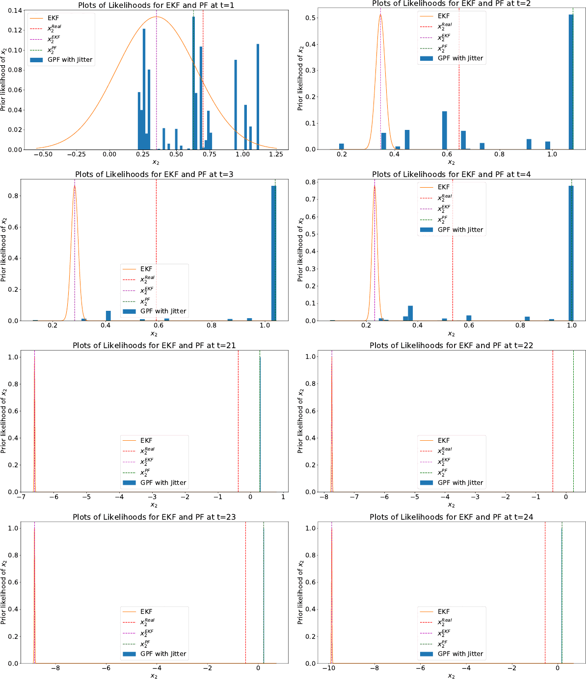
Figure 8, report page 19: the posterior over () at steps 1–4 and 21–24. Bars are particles weighted by ; the curve is the EKF’s Gaussian scaled to the tallest bar; dashed lines are the truth, the EKF mean and the heaviest particle.
Read the top four panels. At the prior is wide and the histogram is a scatter of survivors. By the cloud has two clear clusters (one around , one around ) and the EKF’s Gaussian has picked the near one. The truth (red) is at and then : between them. Neither filter is right at or ; the heaviest particle is on the far cluster and the EKF on the near one. The difference is that the cloud is still holding both stories, and the EKF has already told one and shrunk its covariance to match. Twenty steps later the bottom row shows what that cost: the EKF’s mean has run off to , then , , (the branch cut, then divergence), while the particles are within of the truth.
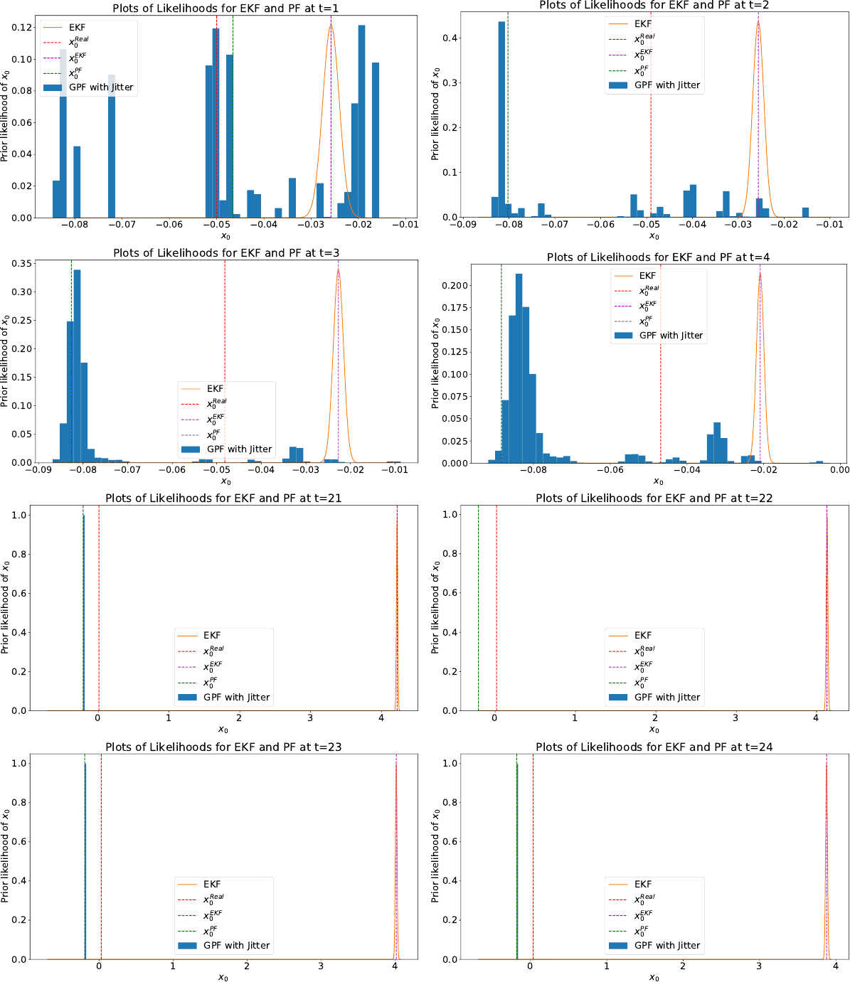
Figure 6, report page 17: the same over (). The multiple clusters at – are the range ambiguity seen along ; the last row is the EKF at after the branch cut.
Figures 7 and 9 (pages 18 and 20) are the two velocity components and tell the same story more quietly; they are in the asset directory if you want them. The report’s discussion, §7, gives the plain-English version that I still think is the right one: the further the initial location is from the starting position, the faster the object would have to move to make a change in the measured angle. This could cause many modes, as the object could be moving very slowly and close, or fast and far away. A particle filter can hold that. A Gaussian cannot.
The lighthouse keeper, with four thousand guesses
Everything above is one scene with a few thousand dots on it, so here is the scene. The bay from post 17, a lighthouse on the headland that measures bearing only (with by default, the report’s is a very good sensor), a ship you steer, a particle cloud coloured by log-weight, and the EKF’s 95% ellipse for comparison. Under the chart: the meter, a weighted histogram in the style of Experiment 4 (pick the axis: range from the light is the one where the modes live), and both filters’ running RMSE. The lighthouse scene is this post’s illustration, not something from the report; the dataset B replay is the report’s problem exactly.
The set-piece. The default prior is two lanes: the keeper knows ships come either along the inshore lane or the offshore one, so half the particles start close and slow and half far and fast, on the same bearing. The inshore cluster is the offshore one scaled toward the light by , velocity included, which makes the bearings identical. The EKF is handed the only thing a Gaussian can hold, the mixture’s mean and spread, and sits between the lanes on neither.
- Press Play with SIS. Both clusters survive. The heaviest particle flickers between them, the range histogram stays two-humped, and collapses to a handful of particles within a few bearings: that is degeneracy. The EKF’s ellipse stretches along the bearing (range is unobservable) and its mean drifts wherever the linearisation takes it.
- Press Resample now. One hump dies. Which one is a coin toss weighted by whichever cluster happened to hold more weight at that instant, and it is not necessarily the wrong one: from a single fixed light there is no evidence to choose. That is the report’s argument for why SIR has the largest upper bound on this problem: resampling spends the particles that would let you recover. Switch to GPF and it happens on its own the first time ; switch to SIR and it happens every step.
- Switch on the second lighthouse. Two bearings intersect at a point. The cloud collapses onto the truth within a step or two and the EKF’s ellipse snaps shut with it, the same thing §6.7 and Table 3 of the report show when a range measurement is added to dataset B and the EKF becomes usable again ( against the best particle filter’s , still worse but no longer a different order of magnitude). Drag either light around and watch the intersection geometry matter: two lights close together are nearly one light.
- Turn jitter on, then set to 100. With a hundred particles and no jitter the cloud is a handful of copies after the first resample; with jitter it stays a cloud. Slide to 10 000 and the histogram becomes the smooth two-humped posterior the maths promised.
The replay. Switch the scene to Dataset B replay and you get the report’s problem with the report’s numbers: 24 steps, , GPF with jitter as in Experiment 4, the sensor at the origin, the report’s , , and starting points. Step through it and watch the bearing sweep past the sensor around step 12; the error₄ readouts are the harness’s mean-over-four-states squared error, directly comparable with Table 2. Run 20 replays averages fresh runs so you can reproduce the table’s order of magnitude in a second or two, and the wrap bearing innovation toggle is the branch-cut fix from the caveat above.
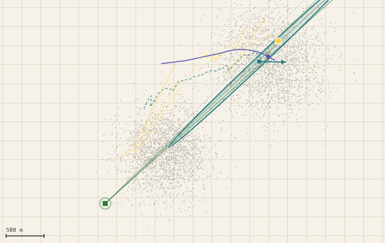
With JavaScript on, this is a live particle filter: steer the ship with the arrow keys, switch between SIS, GPF and SIR, add jitter, set the particle count from 100 to 10 000, press Resample to watch a mode die, add a second lighthouse to resolve the ambiguity, or replay the report’s dataset B and reproduce Table 2.
How the widget differs from the Python
The port is the algorithms above on one flat Float64Array of length with the
log-weights in another: no object per particle, nothing allocated after construction.
Four differences from the Python, each marked DIFFERS: in the source:
-
Systematic resampling instead of
np.random.choice. One uniform draw, evenly spaced pointers, one pass over the cumulative weights: and lower-variance than independent multinomial draws.const u0 = rng.next() / n; let j = 0; for (let i = 0; i < n; i++) { const u = u0 + i / n; while (w[j] < u) j++; // w holds the cumulative weights xs.set(x.subarray(4 * j, 4 * j + 4), 4 * i); } -
Weights reset to after a resample.
ParticalFilterGenerickeepsself.logw[ind](the chosen particles’ old weights) and renormalises, so a heavy particle is duplicated and stays heavy. Algorithm 6 leaves the post-resample weights unstated; uniform is what the operation means. -
Jitter as , per the caveat above.
-
A wrap toggle on the bearing innovation, off in the replay so the numbers match the table, on in the lighthouse scene because a keeper would not report a change of bearing.
The EKF is a compact bearings-only filter built the same way: Algorithms 1 and 2 with
TestProblem3’s Jacobians and a row of per lighthouse, on the shared
engine’s matrix helpers. The ship, the clock, the panel and the world canvas are the
same world-sim engine posts 17 and 18 use.
Performance
The plan’s arithmetic holds: ten thousand particles × four states × sixty frames a
second is about ten million flops a second, which is nothing. The two things that would
have made it slow are avoided. The cloud is drawn by writing pixels into one ImageData
and blitting it once (four thousand arc() calls a frame is the classic mistake), and
the per-step work (predict, weigh, log-sum-exp, resample) touches each particle a
constant number of times with no allocation. Measured in headless Chrome at 1280 px wide,
one simulation step plus one full redraw takes 3–4 ms at and 5–6 ms
at , against a 16.7 ms frame budget; the twenty-replay batch
(20 × 24 steps × 4000 particles) runs in about 0.8 s. WebAssembly is not
needed here and would have been a distraction. It would be the answer at particles,
where the weighing loop alone starts to eat the frame; that is the post-20 territory of
sweeping and starting positions over thousands of Monte-Carlo runs.
What I would say now
The report’s discussion, §7, makes four points I still agree with, and I would add one.
The EKF wins on dataset A because is simple, the first-order approximation is accurate, and there is one mode; it loses on dataset B because there are several, and the particle filter is able to recover if it has diverged to the wrong state vector, as a single particle left in a region of lower probability is able to assist the algorithm to recover from its mistake. That is why SIS, which never throws a particle away, was the best of the six on this problem and SIR, which throws them away every step, had the widest spread.
Particle filters cost more per step, but every particle is independent, so they parallelise across cores and GPUs in a way the Kalman filter’s matrix inverse does not; and they spend their computation where the posterior is, not uniformly over the state space.
The number of particles is a knob with a decaying-exponential payoff (§6.6 sweeps it), and 4000 was enough for dataset B. And the closer and faster the target, the fewer alternative stories fit the bearings, so the better the EKF does; the far-and-slow ambiguity is what kills it.
What I would add is the thing the widget makes physical: no amount of filtering fixes an unobservable problem. From one fixed lighthouse, range is not in the data, and the “multi-modality” is the posterior accurately reporting that. A particle filter’s real virtue here is that it keeps saying so (the cloud stays two-humped) until something in the data, a second bearing or a manoeuvre by the observer, resolves it. The EKF’s failure is not that it gets the answer wrong. It is that it reports a small ellipse around a wrong answer and stops listening.