Blog · Handwritten digits ·
Histogram of Oriented Gradients, from scratch
The one hand-designed feature that scores above 0.90 information gain on every MNIST digit: what it computes, why orientation beats position, and a live rose-overlay visualiser.
- interactive
- computer-vision
- feature-engineering
- hog
- mnist
- wasm
The last post went through three hand-designed features for the MNIST naive-Bayes classifier (arc length, enclosed area, contour count) and none of them was good at more than one or two digits. Arc length picks out 1s. Enclosed area picks out 0s. Everything else, it shrugs at. This post is about the feature that didn’t shrug: Histogram of Oriented Gradients (HOG) scores an information gain above 0.90 for every single digit, and the report says so outright:
This feature yields excellent results and could even be used by itself.
That is not a small claim: it is the reason the whole classifier works as well as it does. This post explains what HOG actually computes, reproduces the repo’s own 24-vs-48-vs-96-dimension decision, and ships a live visualiser: the classic HOG “rose” overlay, over a synthetic street scene (the case HOG was actually built for), an MNIST digit, a drawing, an upload, or the camera.
The pipeline
HOG’s idea is simple to state and easy to get wrong in the details. Take the gradient (magnitude and direction) at every pixel. Group pixels into small square cells. Within a cell, build a histogram of gradient directions, each pixel voting with a weight equal to its gradient magnitude. Group cells into blocks, and normalise each block’s histogram so it is not thrown off by contrast or how hard someone pressed the pen. Glue every block’s normalised histogram together, and that concatenation is the descriptor.
The gradient at pixel comes from the two axis derivatives:
Dalal & Triggs, who introduced HOG for pedestrian detection in 2005, tried several
gradient kernels (including 3×3 and 5×5 Sobel) and found this plain, un-smoothed
[-1, 0, 1] mask worked better, not worse: smoothing throws away exactly the
fine edge information HOG depends on. Each pixel’s vote is split between the two nearest
orientation bins by linear interpolation (soft binning), rather than dumped entirely
into one, with 30°-wide bins, a pixel at 44° mostly votes for the 30–60° bin but leaves a
little in the 60–90° one, so the histogram does not jump around as gradients drift across
a bin boundary. A cell’s histogram is numbers, one per orientation bin; a block of cells is numbers before normalisation.
Why normalise per block
A stroke drawn hard and dark has bigger gradient magnitudes than the same stroke drawn lightly: same shape, different histogram, if you stop after the cell step. Block normalisation is what throws that difference away. Each block’s histogram vector is L2-Hys normalised: L2-normalise, clip every component to a threshold, then L2-normalise again:
where is the clip threshold set in the repo’s own config, L2HysThreshold. The clip
stops one very strong edge from swamping every other bin in its
block after the first normalisation; the second pass re-normalises after clipping. The
widget’s brightness slider and “un-normalised alongside” toggle exist to make this
argument something you drag, not something you take on faith.
The repo’s configuration
The descriptor-generation script builds the descriptor with OpenCV’s cv2.HOGDescriptor, not
hand-rolled code, worth saying plainly, since the repo leans on the library here the way
it leans on cv2.findContours and cv2.minAreaRect in the previous post. Its config:
winSize = (32,32)
blockSize = (16,16)
blockStride = (16,16)
#cellSize = (8,8)
cellSize = (16,16)
#nbins = 3
nbins=6
Then, after warping each digit to a canonical 32×32 window (the deskew from the previous post):
hist = hog.compute(bigImg,winStride,padding,locations)
for i,hel in enumerate(hist):
    outputDescriptor["HOG"+str(i)]=float(hel[0])
Work through the arithmetic and it’s satisfying: a
32×32 window with 16×16 cells is a 2×2 grid of cells. blockSize == cellSize, so each
block is exactly one cell: no cell is shared between blocks. blockStride == blockSize,
so blocks tile the window with no overlap: 2×2 = 4 of them. Four blocks, six bins each,
one cell per block:
Two lines are commented out. Uncomment cellSize = (8,8) on its own and the window
becomes a 4×4 grid of cells; each 16×16 block now covers 2×2 = 4 of them, and there are
still 4 non-overlapping blocks: dimensions. Uncomment
nbins = 3 on its own, instead, with cellSize left at 16×16, and the block count and
shape don’t change at all: only the bin count does: .
Uncomment both together (the repo’s two commented-out lines,
combined) and it’s . Twenty-four, forty-eight,
ninety-six: three sizes sitting in the same eleven lines of code, one uncomment away from
each other. The widget’s three “reproduce the repo” buttons below set exactly these three
configurations, on a real 32×32 MNIST sample, and the live dimensionality readout is
computed the same way this post’s own implementation checks it in its own tests: block
count times cells per block times bins, for the repo’s shipped configuration and both
commented-out ones.
Worth noticing: that sweep trains and scores using HOG alone, no arc length, no enclosed area, nothing else. It exists specifically to answer “how good is this one feature by itself”, which is exactly the question the post opened with.
The information-gain numbers
The report measures every feature the same way: Kononenko’s information gain, base-10 so it’s bounded at 1,
which measures how much predicting class from the feature’s prediction beats knowing nothing at all. Run it over HOG’s 24 dimensions and every one of the ten digits clears 0.90:
| Digit | Information gain |
|---|---|
| 0 | 0.9726 |
| 1 | 0.9185 |
| 2 | 0.9057 |
| 3 | 0.9295 |
| 4 | 0.9652 |
| 5 | 0.9920 |
| 6 | 0.9926 |
| 7 | 0.9480 |
| 8 | 0.9046 |
| 9 | 0.9096 |
The lowest score belongs to the digit ‘8’ at 0.9046, still comfortably above 0.90. Compare that to the previous post’s features: arc length peaked at 0.863 (digit 1) and dropped to 0.163 (digit 8); enclosed area peaked at 0.914 (digit 0) and went negative at −0.004 (digit 3), meaning it did slightly worse than a coin flip once you condition on it predicting a 3. The report puts it bluntly: “These features provided minimal information gain when compared to the HOG descriptor and the moments of the image.” HOG isn’t a good feature among several: on this dataset, it’s carrying almost the whole classifier by itself.
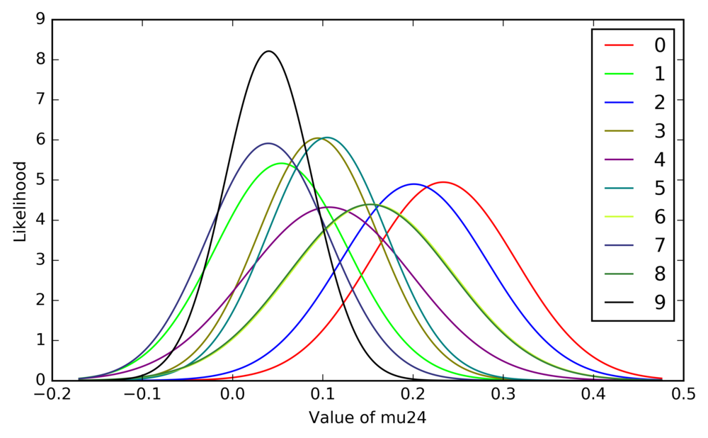
A figure from the report: one HOG dimension’s ten per-class Gaussians, fit and drawn by the report’s own feature-analysis code. Class 9 (black) sits in a narrow, tall peak well separated from the other nine, broader curves. On this one dimension alone, that shape is most of the separating power a naive-Bayes classifier needs. A real figure from the report, cropped and recompressed, not redrawn.
Each of the 24 (or 48, or 96) HOG dimensions gets treated as its own independent Gaussian feature, one per class, the same continuous-feature machinery the next post’s naive Bayes classifier uses for every feature, HOG included. That independence assumption is exactly where naive Bayes earns its name: neighbouring HOG bins genuinely are correlated (a strong edge at 30° usually comes with some weight at 60° too, from the soft binning above), and treating 24 correlated numbers as 24 independent ones is mathematically wrong. It is also why the isolated-HOG classifier in that sweep script doesn’t hit Ebrahimzadeh’s 97.25%: that number comes from HOG paired with a stronger classifier than naive Bayes. 97.25% is the ceiling this feature can reach; naive Bayes, with its independence assumption, won’t get there off HOG alone. The next post in this series measures how close it gets.
An independent Rust port, not OpenCV
The repo computes HOG with cv2.HOGDescriptor, the library, not hand-rolled code. This
post’s widget runs its own implementation, written to explain the algorithm rather than to
match OpenCV byte-for-byte, and it differs in three ways worth naming rather than glossing
over:
- No spatial Gaussian weighting. OpenCV weights every pixel’s vote by a Gaussian
centred on the block (
winSigma = 4.in the repo’s config) before it lands in a cell. This implementation votes every pixel in a cell equally. - Orientation-only interpolation. OpenCV does trilinear interpolation: a pixel’s vote spreads over its two nearest orientation bins and its two nearest cells in each spatial direction. This implementation interpolates orientation only; cell membership is hard-edged.
- Single channel. The repo’s
hog.computeruns on an already-grayscale MNIST digit, so it never had to choose a colour rule. Dalal & Triggs’ original paper takes the maximum gradient across RGB channels for colour images, moot for MNIST, but a real choice for the widget’s street-scene and upload paths, which this port doesn’t make (everything is converted to luma first).
None of that changes the descriptor’s length: the block-count arithmetic above is exact, which is what lets the “reproduce the repo” preset buttons hit 24, 48 and 96 exactly, but the values in this port’s descriptor will not match OpenCV’s bit for bit. This implementation’s own test suite covers the parts that should hold regardless: a gradient at a known angle lands in the expected bin (split correctly between two bins at a 45° boundary), L2-Hys normalisation is invariant to a global brightness scale where the raw histogram is not, and the dimensionality formula matches OpenCV’s block-counting exactly for the repo’s shipped config and both commented-out ones.
Try it
Pick a source: the synthetic street scene below is the case HOG was actually built for (Dalal & Triggs, Histograms of Oriented Gradients for Human Detection, CVPR 2005: strong, consistently-oriented edges along a body’s silhouette are close to invariant across lighting and clothing texture, which is a much harder problem than centred, size-normalised digits). Or pick an MNIST digit from the repo’s own domain, draw something, upload a picture, or use the camera. Drag cell size, bin count, block shape and stride, and watch the dimensionality count update live. Turn on “un-normalised alongside” and drag brightness: the un-normalised rose grows and shrinks with it, the L2-Hys one barely moves. That comparison is the argument for block normalisation, everything above is just the arithmetic behind why.
With JavaScript enabled this becomes a live HOG visualiser: a canvas showing the classic HOG “rose” overlay: every cell drawn as a star of line segments, one per orientation bin, length proportional to that bin’s weight, over a dimmed source image. Pick a synthetic street scene, an MNIST digit from the repo’s own domain, a drawing, an upload or the camera; drag cell size, bin count, block shape and stride and watch the descriptor’s dimensionality update live; toggle a side-by-side un-normalised vs. L2-Hys-normalised comparison and drag a brightness slider to see why block normalisation matters; and export the descriptor as JSON or CSV.
The export button writes exactly what this port’s HOG computation returns: the
block-normalised descriptor, block-major then cell-within-block then bin, the same layout
OpenCV’s hog.compute() hands back, just from this post’s own Rust instead of OpenCV.
Next in this series: naive Bayes, which puts HOG back together with the previous post’s weaker features and asks how far a classifier that assumes every feature is independent can get.