Blog · Handwritten digits ·
Teaching a computer to read by hand: feature engineering for OCR
Before deep learning ate OCR, you told the computer what to look at. Arc length, enclosed area, contour count: three small hypotheses about what makes a digit that digit, scored with Kononenko's information gain.
- interactive
- ocr
- feature-engineering
- information-gain
- mnist
- wasm
Before you can classify a handwritten digit you have to describe it, and in 2018 “describe it” meant deciding, by hand, what to measure. Not a convolution stack that learns its own descriptors: a list of numbers I chose myself, out of a hunch about what makes a “1” a “1” and an “8” an “8”. This is the assignment where I found out how much of that hunch survives contact with 10,000 real handwritten test digits, and where a formula called Kononenko’s information gain turned “I think this feature is useful” into a number I could argue with.

A sample of digits 0–9 from the MNIST dataset: the raw material every feature below is measured on.
The pipeline, once, before the features
Every feature in this post is computed by the same short script, reading straight through
the MNIST idx files. It thresholds, finds contours, measures them, and
warps the result to a canonical size, all with OpenCV, since this was an assignment about
Bayesian classification, not about re-deriving findContours. The canonicalisation step
in particular is easy to skim past and easy to forget is even happening, so it gets its own
section before the features that depend on it.
Threshold, then find contours
ret,threshImage = cv2.threshold(image,20,255,cv2.THRESH_BINARY)
im2, contours, hierarchy = cv2.findContours(threshImage,cv2.RETR_TREE,cv2.CHAIN_APPROX_SIMPLE)

outputDescriptor={"classLabel":lbl}

maxContour=max(contours,key=cv2.contourArea)

outputDescriptor["pixelCount"]=cv2.contourArea(maxContour)
outputDescriptor["arkLen"]=cv2.arcLength(maxContour, False)
A pixel counts as ink once its intensity clears 20.
MNIST backgrounds are flat black, so this threshold has very little work to do. Every
contour in the thresholded image gets found with RETR_TREE (full nesting hierarchy,
compressed to straight-run vertices with CHAIN_APPROX_SIMPLE), and the single largest one
by area becomes “the” contour for the two features that follow.
The canonicalisation step everyone forgets
rect = cv2.minAreaRect(maxContour)
box = order_points(cv2.boxPoints(rect))

dst = np.array([[0, 0],[31, 0],[31, 31],[0, 31]], dtype = "float32")

M = cv2.getPerspectiveTransform(box, dst)
bigImg = cv2.warpPerspective(image, M, (32, 32))

moments=cv2.moments(bigImg, binaryImage=False)
minAreaRect fits the tightest rotated rectangle around the largest contour;
order_points (a routine borrowed from a well-known
PyImageSearch post
and credited to it in a code comment) sorts its four corners into top-left, top-right,
bottom-right, bottom-left by the sum and difference of their
coordinates; and a perspective warp maps that rotated box onto a fixed 32×32 square. Every
downstream feature that touches bigImg (the image moments, the Hu moments, HOG) is
measured on this deskewed, size-normalised digit, not the raw 28×28 one. It is the single
most consequential ten lines in the file and the easiest to miss on a first read, because
nothing about it produces a headline number of its own.
Kononenko’s information gain
Before the features themselves, the yardstick they’re all measured against. Given a feature and a class , the information gain is
Base 2 is conventional (it’s “bits of information gained”) but the report uses , the number of classes, specifically so that and the number reads directly as a fraction of maximum possible gain. Expressed against a predicted class rather than the feature value directly:
A feature that tells you nothing beyond the class base rate scores 0. A feature that is worse than knowing nothing (one whose value, for a given predicted class, actually makes the true class less likely than the prior) scores negative. That second case shows up more than once below, and it’s the more interesting failure mode: not “no signal” but “actively misleading signal,” which is a different bug to go looking for.
Arc length
The hypothesis: a “1” has a short stroke, other digits don’t, so this should split “1” from everything else cleanly. Because the distribution is multi-modal (a “5” written as two strokes versus one continuous stroke are genuinely different shapes with the same label), the report bins the values rather than fitting a single Gaussian per class.
| Class | Class | |||
|---|---|---|---|---|
| 0 | 0.4724 | 5 | 0.7012 | |
| 1 | 0.8630 | 6 | 0.3529 | |
| 2 | 0.3641 | 7 | 0.4001 | |
| 3 | 0.5294 | 8 | 0.1622 | |
| 4 | 0.3066 | 9 | 0.4824 |
The “1” hypothesis holds up: 0.863 is the highest score any of this post’s three features gets, on any class. “5” does well too, at 0.701: not because a “5” is short, but because it’s consistently one length, in contrast to a “4”, which the report calls out by name as the confusable neighbour: a “5” always resolves to roughly the same continuous stroke, while a “4” is drawn with wildly different numbers of strokes and crossings depending on handwriting style, so its arc length is all over the place and tells you comparatively little.
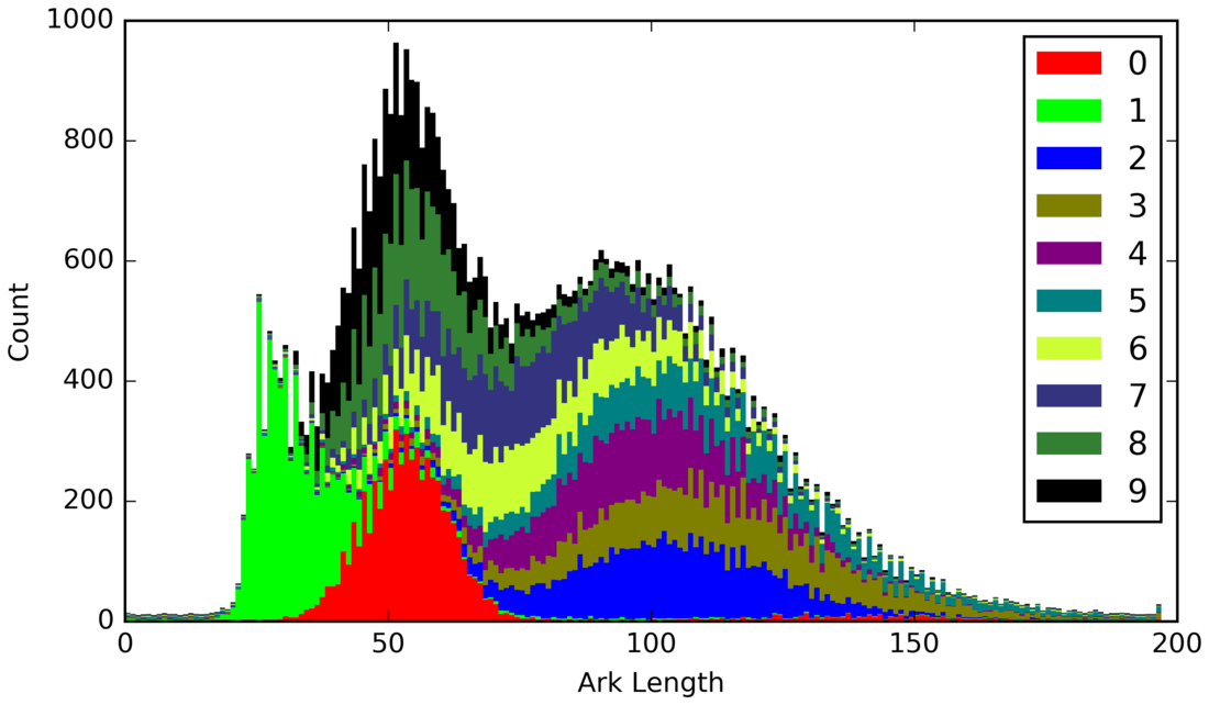
Arc length binned against class counts: the “1” spike sits almost entirely in the short-arc bins.
Area enclosed
The next feature asks a different question: how much background does the ink surround?
The same script answers it by re-running findContours, throwing away anything implausibly
small or large, and summing what’s left:
im2, invContours, hierarchy = cv2.findContours(threshImage,cv2.RETR_TREE,cv2.CHAIN_APPROX_SIMPLE)

for i,cnt in reversed(list(enumerate(invContours))):
    cntarea=cv2.contourArea(cnt)
    if cntarea>700 or cntarea < 2:
        invContours.pop(i)

outputDescriptor["numValidContours"]=len(invContours)

maxVal=0
TotalSum=0
for cont in invContours:
    area=cv2.contourArea(cont)
    TotalSum+=area
    maxVal=maxVal if maxVal > area else area
outputDescriptor["areaEnclosed"]=TotalSum-maxVal
On a 28×28 image the giant outer contour tracing the whole ink blob comfortably clears the 700-pixel ceiling and gets filtered out, leaving mostly the small interior loops: the holes in a “0”, a “6”, an “8”, a “9”. Subtracting the single largest of what’s left from the sum is a quiet detail: for a digit with exactly one hole (a “0”), that leaves 0, which looks wrong until you notice the next feature is built from exactly that count.

What “area enclosed” is measuring, made visible.
| Class | Class | |||
|---|---|---|---|---|
| 0 | 0.9143 | 5 | 0.0491 | |
| 1 | 0.2468 | 6 | 0.5271 | |
| 2 | 0.2845 | 7 | 0.1131 | |
| 3 | −0.0043 | 8 | 0.5912 | |
| 4 | −0.0336 | 9 | 0.5291 |
Both extremes here were checked directly against the report’s own source before quoting them, rather than trusting a rounded summary. This is the payoff of the whole exercise, in one table. 0.9143 for “0”: a zero is, almost by definition, a loop, and this feature measures exactly that loop’s interior. −0.0043 for “3”: a three encloses nothing, a four encloses nothing, so both collapse into the same “zero pixels enclosed” bin as every other non-looping digit, and a feature that can’t tell a “3” from a “7” or a “1” this way is worse than the class prior, not merely unhelpful. Same intuition, confirmed for zeros and quietly falsified for threes, by the same number.
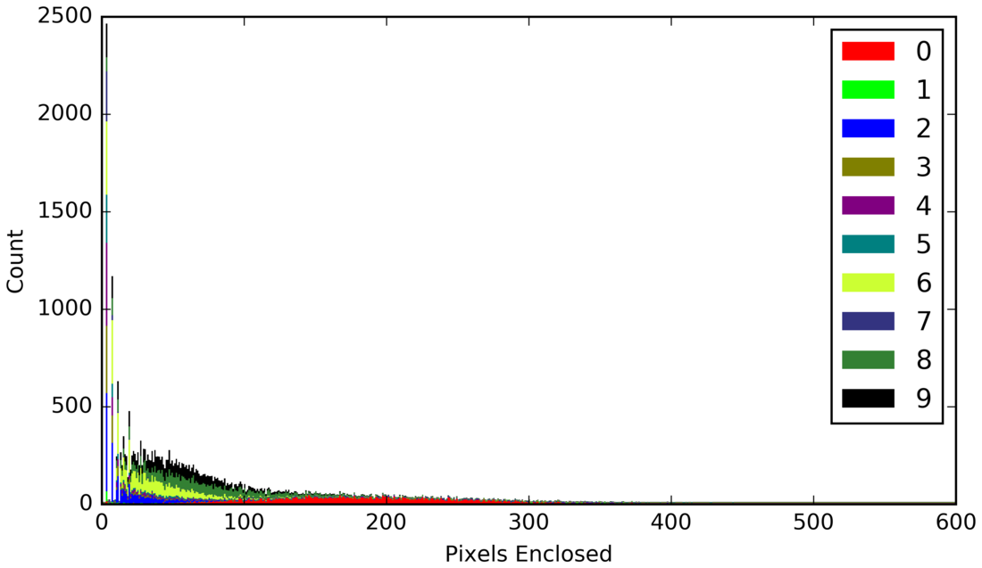
Area enclosed, binned. The zero-pixel bin is removed from the plot, since it held most of the data.
Number of contours
The same filtered contour list from above, counted rather than summed, aimed at one specific confusion: 3 and 8 look alike to a lot of hand-built descriptors, and an “8” has two holes where a “3” has none.
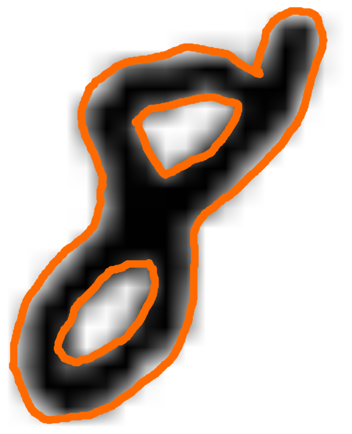
Three contours on one “8”: the outer silhouette plus both interior loops.
| Class | Class | |||
|---|---|---|---|---|
| 0 | 0.4631 | 5 | 0.0491 | |
| 1 | 0.2472 | 6 | 0.0184 | |
| 2 | −0.0135 | 7 | −0.0119 | |
| 3 | −0.0043 | 8 | 0.7254 | |
| 4 | −0.0078 | 9 | −0.0039 |
It is a genuinely single-purpose feature (everything except 0, 1 and 8 scores at or below zero) and it works exactly where it was aimed: 0.725 for “8”, built for the specific job of separating “8” from “3”, with essentially no signal anywhere else. A narrow, built-to-order feature that does its one job is still a good feature; it just isn’t a general one, and the classifier needs several of these stacked together rather than one that does everything.
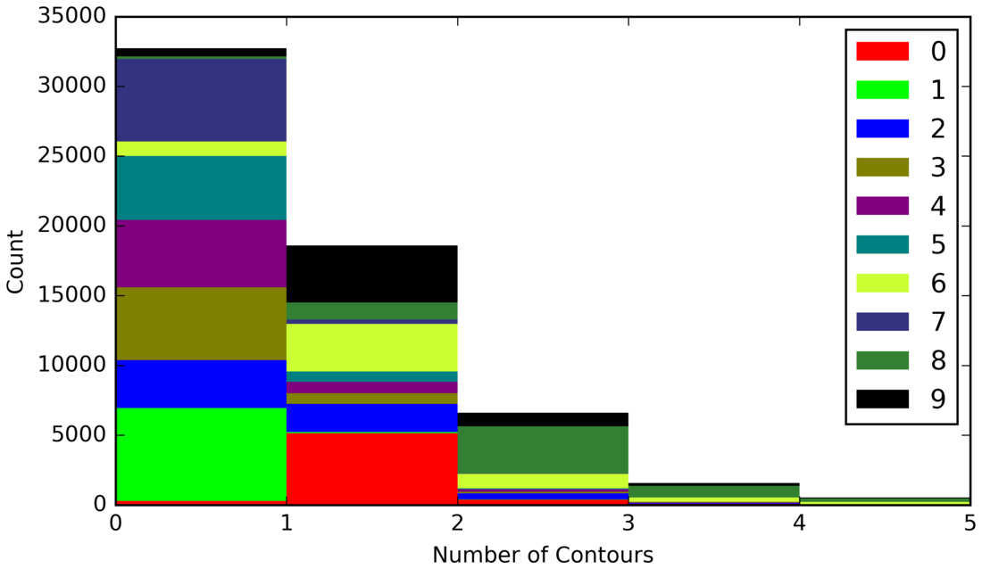
Contour count, binned.
The features that don’t get their own write-up
The same script computes considerably more than these three. Alongside arc
length, area enclosed and contour count, it extracts the raw contour pixel count, the
minAreaRect’s own length/width/area, seven Hu moments and eight raw image moments, a
Harris corner count, and horizontal/vertical Hough line counts. Every one of them is
loaded back by the training script and the evaluation script downstream, and used to build
the trained classifier. They just don’t get the same
information-gain write-up in the report’s prose that arc length, area enclosed, contour
count and HOG (next post) do. HOG in particular is worth flagging now and coming back to:
its worst per-class information gain, 0.905, beats this post’s best number by a
comfortable margin: the report says outright it “could even be used by itself.” That’s
the next post.
Hough lines, with a bug
lines = cv2.HoughLines(threshImage,1,np.pi/180,13)
# ...classify each detected line as roughly horizontal or vertical...
    outputDescriptor["HLines"]=len(VLines)
    outputDescriptor["VLines"]=len(HLines)
Read that assignment again and it’s an easy one to miss: the variable holding
near-vertical lines gets written out under the JSON key "HLines", and the variable
holding near-horizontal lines gets written out under "VLines". Every trained model
built from this script’s output has had its horizontal and vertical line counts swapped,
silently, at the point of serialisation.
It’s a fun one to find years later: trivial to catch by eye on a single digit, and easy to
miss forever in a training pipeline that never looks at the raw numbers again.
Harris corners
cornerImg = cv2.cornerHarris(255-image,2,1,0.14)
corners=np.argwhere(cornerImg > 0.02)
# ...deduplicate points within 3px of one another...
outputDescriptor["cornerCount"]=len(corners)
Corners on the inverted image (bright background, dark ink) with a small 2×2 block, an aperture-1 Sobel (a plain central difference, no smoothing pass), sensitivity , and a de-duplication pass that discards any corner within 3 pixels of one already kept: the exact clustering logic my own implementation reuses below.
What the widget builds, and where it diverges from OpenCV
The crate implements Moore-neighbour contour tracing, a scanline flood fill, a
rotating-calipers minimum-area rectangle, and the
perspective warp with bilinear sampling, all from scratch, no imageproc, no OpenCV. It
gets close, not identical, and getting exactly identical was always going to be the hard
part, so here’s where the two line up and where they don’t:
- Contours. OpenCV’s
RETR_TREEbuilds a full nesting hierarchy in one pass. This crate instead traces outer boundaries of ink components with a textbook Moore-neighbour tracer, and finds holes independently with a scanline flood fill of the background, checking which background regions never touch the image border. For every digit shape (no ink island sitting inside a hole sitting inside more ink) the two answers agree. A shape with three-deep nesting would not be represented correctly; MNIST digits never have one. - Arc length. Measured on the raw 8-connected boundary chain rather than OpenCV’s
CHAIN_APPROX_SIMPLE-compressed one. Removing collinear interior points from a straight run doesn’t change that run’s total Euclidean length, so the two should agree to floating-point rounding. I haven’t run this against the report’s own quoted distribution to confirm the bin-by-bin fit, so I won’t claim more than that. - Area enclosed. Where the report sums
contourArea(a shoelace-formula polygon area) over small hole contours, the widget counts flood-filled pixels directly. Conceptually the same question (how much does this digit’s ink enclose?) answered a different way, and the numbers won’t match exactly pixel for pixel against a polygon area. - Harris and Hough are standard textbook implementations, tuned by eye rather than against the report’s exact numeric response scale. Neither gets its own information-gain section above, so exact agreement wasn’t the goal: a reasonable corner or line count was.
I’d rather say precisely where the fidelity ends than claim a match I didn’t verify.
With JavaScript enabled, this becomes a live pipeline: draw a digit (or upload, paste, or load an MNIST sample), and watch it get thresholded, contour-traced, flood-filled for enclosed area, fitted with a minimum-area rectangle, deskewed to the canonical 32×32, and scored against the report’s real per-class information gain, all running in Rust compiled to WebAssembly, in this page, on your input.
Draw a wonky, off-axis “7” and watch the minAreaRect panel and the deskewed 32×32 next to
it: that’s the moment the canonicalisation section above stops being an abstract ten lines
of Python and starts being a picture. The three gauges below the contour panels place your
digit’s own arc length, enclosed area and contour count on the report’s real bin ranges
next to its real per-class information gain; untick a feature
to grey it out of the combined chart and see how much of the picture that feature alone
was carrying. “Export feature vector” writes out exactly the numbers the next post’s
classifier will want.
What’s next
Arc length, area enclosed and contour count get this post’s full information-gain treatment because they’re small, explainable, hand-built hypotheses: each one a single sentence of “I think this measures X.” The next post is the opposite kind of feature: the Histogram of Oriented Gradients, which scores above 0.90 for every class simultaneously and doesn’t reduce to a one-line intuition nearly as easily. Both feed the same naive Bayes classifier, in the post after that.