FERN: feature matching as a classification problem

The last post took a correspondence for granted: two matched keypoints went in, z = bf/d came out. This one is about finding the correspondence in the first place, and it does it in a way most descriptors don’t. SIFT and SURF compute a vector per keypoint and compare vectors by distance. FERN never computes a vector at all: every reference keypoint is a class, and matching a patch means answering “which class is this?”, the same question a classifier answers, with a few hundred one-bit questions of the form is pixel A brighter than pixel B? standing in for the usual gradient histogram.

Matching as classification

Report page 19 (docs/pngs/report-19.png) is close to a complete tutorial on its own, so it’s transcribed and rephrased below rather than cropped: the honesty rule for this series is that prose and equations get retyped in my own voice, never pasted as an image.

FERN (Ozuysal, Fua and Lepetit, CVPR 2007 [12]) treats every keypoint the classifier was trained on as a class $c_i$ . Given $N$ binary features $f_1, \dots, f_N$ measured at a candidate location, the question is which class most plausibly produced them. With Bayes’ rule and a uniform prior over classes, the report’s Eq. 5.2:

\hat c = \operatorname*{argmax}_{c_i} P(f_1, f_2, f_3, \dots, f_N \mid C = c_i)

Each feature is one comparison between two pixels, offset from the keypoint by a fixed, randomly chosen pair of displacements $\mathbf{d}_{i,1}, \mathbf{d}_{i,2}$ , Eq. 5.3:

f_i = \begin{cases} 1 & \text{if } I(\mathbf{d}_{i,1}) < I(\mathbf{d}_{i,2}) \\ 0 & \text{otherwise} \end{cases}

The offsets are drawn once from a zero-mean Gaussian, $\sigma = 4$ px in this implementation, and reused for every keypoint and every match: “the Gaussian distribution was chosen as it is rotationally symmetric [and] sets most of the descriptor points close to the feature,” weighting nearby pixels more heavily without having to say so explicitly. Fern_Detector_Class.py:21:

self.D = np.random.normal(0, sigma_d, [2, 2, N]).astype(np.int32)

The wall, and the fern

Estimating $P(f_1, \dots, f_N \mid C)$ directly needs $2^N$ table entries per class: with the paper’s recommended $N \approx 300$ tests, $2^{300}$ , which is not a number. Assuming every test is independent fixes the storage problem and wrecks the accuracy: adjacent brightness comparisons are correlated by the image they’re both looking at, and pretending otherwise throws that structure away.

The fern is the compromise: split the $N$ tests into $M$ groups of $S$ tests each (a “fern” $F$ ) and assume independence between groups while keeping the joint distribution within one group. Eq. 5.4:

P(f_1, f_2, \dots, f_N \mid C = c_i) = \prod_{m=1}^{M} P(F_m \mid C = c_i)

Storage drops to $M \times 2^S$ per class, typically $M \in [30, 50]$ , $S \in [10, 16]$ , a direct dial between accuracy and memory that this implementation exposes as N and S (self.M = self.N // self.S, Fern_Detector_Class.py:15). The default is $N=440$ , $S=11 \Rightarrow M=40$ ferns of $2^{11}=2048$ entries each; the full driver run (test_all_reconstruction.py:91) uses $N=720$ , $S=12$ .

Training estimates every $P(F_m \mid C=c_i)$ by warping the one real view of each keypoint many times and counting which code each fern produces. Eq. 5.5:

P(F_k \mid C = c_i) = \frac{n_{k,i} + u}{\sum_k (n_{k,i} + u)}

$n_{k,i}$ is how many of the training warps produced code $k$ for class $i$ ; $u$ is a Dirichlet/Laplace prior, set to 1: the +1 that keeps a code nobody has seen yet from zeroing out the whole product. train(), Fern_Detector_Class.py:27-53:

def train(self, img):
    self.img_ind = np.indices(img.shape[:-1])
    self.key_points = cv2.AgastFeatureDetector.create().detect(img)
    self.key_points = np.array([(kp.pt[1], kp.pt[0]) for kp in self.key_points if
                                (self.border < kp.pt[0] < img.shape[1] - self.border) and (self.border < kp.pt[1] < img.shape[0] - self.border)],
                               dtype=np.int32).T

    self.C = self.key_points.shape[1]
    self.ind = np.indices((self.C, self.M))
    self.PFk = np.ones((self.M, 2 ** self.S, self.C))

    for i in range(self.Nt):
        warpedD = np.rint(np.dot(self.D.T, self.get_random_transform().T).T).astype(np.int32)
        warped_pts = warpedD[:, :, None, :] + self.key_points[:, None, :, None]

        trainingPoints = (img[np.clip(warped_pts[0], 0, img.shape[0] - 1),
                              np.clip(warped_pts[1], 0, img.shape[1] - 1),
                              self.D_c]
                          + np.random.normal(0, self.sigma_n, (2, 1, self.M * self.S)))

        features = (trainingPoints[0] > trainingPoints[1]).reshape((self.C, self.M, self.S))
        features_i = np.dot(features, self.conversion)
        self.PFk[self.ind[1], features_i, self.ind[0]] += 1
        if i % self.NinPercentage == 0:
            print("Training " + str(100 * i / self.Nt) + "% Complete")

    self.PFk /= self.PFk.sum(axis=(0, 1))

self.PFk starts at np.ones(...), the prior, applied by initialising the count rather than adding it in afterwards, and every one of the Nt warps adds exactly one count to exactly one code, for every fern, for every class simultaneously (self.ind[1]/self.ind[0] broadcast the update over all $M$ ferns and all $C$ classes in one indexed assignment). self.conversion = 2 ** np.arange(self.S) (line 16) is the bit-packing: np.dot(features, conversion) at line 48 turns $S$ booleans into one integer in $[0, 2^S)$ by treating them as the bits of a binary number, least-significant test first: exactly what FernBank’s pack_bits/unpack_bits round-trip against in the crate’s tests.

The rotation that never happens

Report page 19 states the domain-specific choice plainly, and the widget’s whole reason for having a σ-and-rotation story is this paragraph:

“As proposed by V. Lepetit and P. Fua[13], it is possible to decompose the distortion into $\mathbf{R}_\theta \mathbf{R}_\phi^{-1} \mathbf{S} \mathbf{R}_\phi$ . Here $\mathbf{R}_\theta, \mathbf{R}_\phi$ are two rotational matrices and $\mathbf{S} = \operatorname{diag}(\lambda_1, \lambda_2)$ . In the original paper both $\phi$ and $\theta$ are drawn from $[-\pi, \pi]$ . However it was decided to draw $\theta$ from $[-\pi/16, \pi/16]$ as there is not much rotation between the stereo images. This allows a more accurate representation of $P(F_k \mid C=c_i)$ to be modelled, achieving higher accuracies.”

The reasoning is sound and worth keeping: the paper’s random-fern trees were designed for general object recognition, where a keypoint really can turn up at any orientation. Rectified stereo pairs don’t do that (the two cameras differ by a small baseline shift, not a spin), so training the classifier to be invariant to $\pm\pi$ of rotation spends its warping budget modelling distortions that will never occur in a stereo pair, which only blurs the $P(F_k \mid C=c_i)$ the classifier actually needs. Restricting $\theta$ to $\pm\pi/16$ (≈11°) puts that capacity where the real variation is: viewpoint-dependent foreshortening and the small perspective differences between two nearby cameras.

get_random_transform, Fern_Detector_Class.py:76-87:

@staticmethod
def get_random_transform():
    phi = np.random.uniform(-np.pi / 16, np.pi / 16)
    #phi = np.random.uniform(-np.pi / 16, np.pi / 16)
    theta = np.random.uniform(-np.pi / 16, np.pi / 16)
    lambdas = np.random.uniform(0.5, 1.6, 2)

    R_theta = np.array([[np.cos(theta), -np.sin(theta)],
                        [np.sin(theta), np.cos(theta)]])
    R_phi = np.array([[np.cos(phi), -np.sin(phi)],
                      [np.sin(phi), np.cos(phi)]])
    return np.linalg.multi_dot((R_theta, R_phi, lambdas * R_phi.T))

Look closer and my prose and my code disagree on more than they let on. My report says only $\theta$ was restricted from the paper’s $[-\pi,\pi]$ to $[-\pi/16,\pi/16]$ , but the code draws phi from the same restricted range too, on the very next line, with a duplicate commented-out copy of that draw sitting directly above it (line 79): a fossil of me editing this in place at the time and never going back to update the paragraph that describes it.

Caveat

It doesn’t matter, and here’s why. R_phi is a rotation matrix, so $\mathbf{R}_\phi \mathbf{R}_\phi^{\mathsf T} = \mathbf{I}$ for every value of $\phi$ . NumPy’s lambdas * R_phi.T broadcasts the length-2 lambdas vector against the last axis (columns) of R_phi.T, which is exactly $\mathbf{R}_\phi^{\mathsf T} \operatorname{diag}(\boldsymbol\lambda)$ : scaling each column by its own $\lambda$ . So the whole expression the code computes is

\mathbf{R}_\theta \, \mathbf{R}_\phi \left(\boldsymbol\lambda * \mathbf{R}_\phi^{\mathsf T}\right) = \mathbf{R}_\theta \, \mathbf{R}_\phi \, \mathbf{R}_\phi^{\mathsf T} \operatorname{diag}(\boldsymbol\lambda) = \mathbf{R}_\theta \operatorname{diag}(\boldsymbol\lambda)

for any $\phi$ : it cancels exactly, algebraically, not approximately. Every warp this code has ever trained on is a plain rotation by $\theta$ followed by an axis-aligned scale, never the paper’s rotated-shear $\mathbf{R}_\theta \mathbf{R}_\phi^{-1} \mathbf{S}\mathbf{R}_\phi$ . Sampling $\phi$ at all (twice, given the dead duplicate line) spends two random draws per warp on a value that can never affect the output. I checked this two ways: algebraically above, and numerically, evaluating the full NumPy expression against the simplified one for fifty random $(\theta, \phi, \lambda_1, \lambda_2)$ draws in r_theta_diag_lambda_matches_the_full_numpy_expression: they agree to five decimal places every time, for every $\phi$ tried, including ones far outside $\pm\pi/16$ . Working that out was the fun part of porting this to Rust: eight years on, the geometry these models actually learned turns out to be simpler than my own code let on.

My Rust crate’s random_transform computes $\mathbf{R}_\theta \operatorname{diag}(\boldsymbol \lambda)$ directly: the same number the Python produces, with the cancelling detour removed, and no $\phi$ parameter to draw at all.

Fern.py’s dead visualisation, resurrected

Before it became the tidy FERN class above, my earlier draft script built the same pieces top-to-bottom, and I’d left a block commented out that would have drawn exactly what the sampling looks like, Fern.py:36-45:

"""
img_out = cv2.cvtColor(img1, cv2.COLOR_GRAY2BGR)
for i in range(pts.shape[2]):
    c = (np.random.randint(0,255), np.random.randint(0,255), np.random.randint(0,255))
    for j in range(pts.shape[3]):
        cv2.line(img_out, (pts[1,0,i,j], pts[0,0,i,j]), (pts[1,1,i,j], pts[0,1,i,j]), c, 1)

cv2.imshow("img", img_out)
cv2.waitKey(0)
"""

One coloured line per test pair, drawn over the keypoint, colour-per-fern: never run, as far as I can tell from the repo. Stage 1 of the widget below is that exact block, restored and made interactive.

The Rust

wasm/crates/stereo-wasm/src/fern.rs: the crate post 29 started, extended with a fern module rather than touched anywhere else, per the workspace’s own convention for a crate several posts share. cargo test -p stereo-wasm runs 8 tests against it: the bit-packing round-trip, the $\phi$ -cancellation check above, training on warps of one patch correctly peaking that patch’s class, an unseen code never scoring zero, match_line finding the true position along a row, resetting training while keeping the same test offsets, and the keypoint cap. pnpm build:wasm stereo-wasm adds about 16 kB to the shared crate (43.9 kB with fern.rs compiled in against 27.5 kB without it; the surf.rs module post 43 is landing concurrently in the same crate and accounts for the rest of the 58.8 kB the built .wasm currently reports).

Three differences from the NumPy, beyond the $\phi$ simplification already covered:

A second find, this time in my own report's equation

Porting train() turned up a second one. Its normalisation (line 53) is self.PFk /= self.PFk.sum(axis=(0, 1)), summed jointly over every fern and every code for a class, not per fern the way Eq. 5.5 reads. It happens not to matter for classification: every warp adds exactly one count to exactly one code in every fern (self.ind[1] broadcasts the += 1 across all $M$ ferns each iteration), so each fern’s own row always sums to the same constant $2^S + T$ after $T$ warps, regardless of which fern, meaning the joint normalisation is just the correct per-fern one, divided everywhere by the constant $M$ . A constant factor cancels under $\operatorname*{argmax}$ , so the code still classifies correctly. But it does mean the shipped PFk doesn’t actually satisfy the equation it was derived from: ask it to sum over one fern’s $2^S$ codes and you get $1/M$ , not 1. FernBank::posterior in the Rust normalises per fern, so it does; posterior_normalisation_sums_to_one_per_fern is the test.

Grayscale, not a random channel. self.D_c (Fern_Detector_Class.py:22) picks a colour channel at random per test, because the report’s images are colour. The widget’s images are read as luma (fern_rgba_to_gray, Rec. 601 weights: the same ones cost.rs uses for the dense posts), so every test reads the one channel there is.
Shared noise, faithfully kept. train()’s per-test pixel noise (line 45) has shape (2, 1, M*S), one draw per test per warp, broadcast across every class, not independently redrawn per keypoint. FernBank::train_step reproduces this exactly: one random transform and one noise draw per test per warp, shared across every keypoint being trained in that iteration, matching the report’s own arithmetic rather than “fixing” it into something more independent than the source.

Does it work? Table 5

Report page 21 scores FERN on five Middlebury frames with the standard bad- $N$ metric: the percentage of matches whose reprojected point misses ground truth by more than $N$ pixels:

Dataset	Image	ERR1 (%)	ERR2 (%)	ERR3 (%)	ERR5 (%)
cones	2	41.2	30.6	23.5	14.8
cones	6	83.3	70.5	59.5	41.6
teddy	2	43.9	34.1	27.5	21.1
teddy	6	85.1	64.4	56.9	45.7
tsukuba	row 3, col 3	47.0	38.7	34.1	26.4

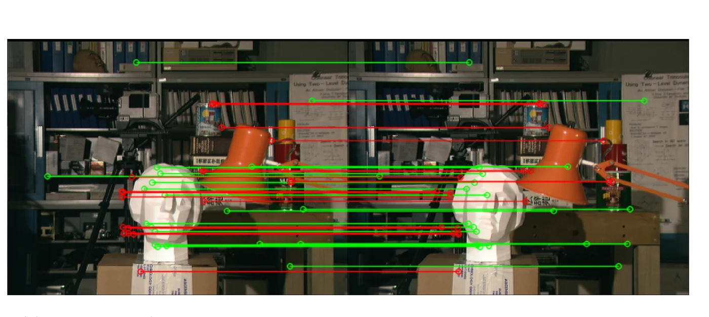
FERN's matches on the Tsukuba pair, drawn as lines between the two images: green lines connect matches within 3 pixels of ground truth, red lines connect matches that missed by more than 3 pixels — Figure 17(a): every point FERN matched between the reference and probe Tsukuba frames, green within 3 px of ground truth, red not. A real figure from the report, not a regenerated plot: the widget scores its own hand-picked keypoints the same way, but this is the actual full-image run that produced Table 5.

The report’s own §5.4 discussion (report-36.png) puts FERN’s number in context against SURF, the descriptor two posts from now will rebuild from the paper up:

“FERN was able to correctly identify more points in the image, however SURF had a higher accuracy rate. This was due to the stricter thresholds on SURF as it allowed fewer but more accurate features to be matched.”

Try it: train ferns and watch a match collapse

FERN matches on the Tsukuba stereo pair — InteractiveFern trainer & matcher

Bundled imagery: no dataset file exists in either stereo repository (see the widget’s own SOURCES.md), so the pair above is a re-crop of the shared report’s own Figure 8, the same approach posts 29 and 32 used: Tsukuba’s reference and third-column views, plus the ground-truth disparity map at its /8 scale (traced through test_all_reconstruction.py’s dataset table, not assumed).

Three things worth doing with it.

Stage 1: watch σ tighten the cloud. Click anywhere in the left image and the widget draws every one of the $N = M \times S$ test-pair segments live, coloured by which fern they belong to. Drag σ down toward 1 and the whole cloud collapses onto the keypoint itself: every test is now comparing two nearly-identical pixels, which is nearly useless. Drag it up past 6 or 7 and the tests start reaching into completely different, unrelated parts of the patch. Four is the report’s own choice for a reason: enough spread to see real structure, not so much that a test stops being about the keypoint at all.

Stage 2: train to 1000 warps, then to 10, on the same keypoint. The bar chart starts flat (every code equally likely, the Dirichlet prior with nothing added yet) and fills in as training runs, live, batch by batch from the worker. At 1000 warps a handful of codes dominate the chart for a well-textured patch. Turn the warp slider down to 10 and retrain: the histogram barely leaves the flat prior, and the M × 2^S storage-cost readout keeps climbing if you push S and M up regardless: the parameters cost memory whether or not training earned them.

Stage 3: match, then break it on purpose. With a trained keypoint, the score plot along the epipolar line usually has one clear peak, and the widget marks whether that argmax lands within 3 px of the crop’s ground-truth disparity, the same ERR3 tolerance Table 5 reports. Go back to stage 2, retrain the same keypoint at 10 warps, and match again: the peak flattens into noise, and the argmax becomes close to arbitrary. That’s Table 5’s ERR columns happening to one point in real time, not summarised over a whole dataset.

What’s next

Two posts from now, SURF, rebuilt from the paper up, takes the other half of §5.1’s comparison (a real descriptor vector instead of a classifier) through the same Tsukuba pair, with a Hessian the original NumPy computes by convolution and this series’ Rust computes by integral image instead.