Blog · Stereo ·
Two images, one depth map
Dense stereo from first principles: why the search collapses to one scanline, what SAD, SSD and ZNCC actually cost, and a live disparity explorer in Rust and WebAssembly where hovering a pixel draws its cost curve.
- interactive
- stereo
- disparity
- block-matching
- zncc
- rust
- wasm
Depth from two photographs is one of those problems that sounds impossible and then turns out to be almost entirely bookkeeping. If you know where the two cameras are, and you can find the same physical point in both pictures, the depth of that point is a division: , baseline times focal length over disparity. The calibration posts already handed me and . So the whole of stereo reduces to one sentence:
Given a pixel in the left image, which pixel in the right image is the same piece of the world?
That is the correspondence problem, and it is the only hard part. This post is the dense answer to it (every pixel gets a match), written up from the two thirty-line NumPy functions that are the whole of it, and rebuilt here in Rust so you can drag the knobs yourself.
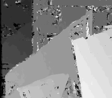
The one disparity map I saved from that run: ZNCC on the Teddy scene’s wide-baseline
pair, im0 against im6. Bright is near. The black speckle is not noise: a match that
fails the accept threshold is written as zero, and zero is black.
The search is two-dimensional, and then it isn’t
Section 4 of the report opens by splitting correspondence into two families, and the split still holds up. Direct or correlation-based methods take a region around a point in the first image and try to match it against regions in the second. Feature-based methods find distinctive points independently in both images and then match descriptors. Direct methods are the ones that give you a depth for every pixel, and they are also the expensive ones, because in the worst case each pixel in the first image has to be compared against every pixel in the second.
The saving grace is epipolar geometry. A point in the left image does not correspond to some arbitrary pixel in the right one, it corresponds to a point on a line, the projection of the ray you are looking along into the other camera. That already turns a 2-D search into a 1-D one. And if the two cameras differ by nothing but a horizontal translation, that line is a horizontal line: the epipolar line is the scanline. Match a pixel at row , column in the left image, and its partner is at row , column in the right image for some non-negative . That is the disparity, and it is the only unknown left.
What this code does not do, and why that was fine
Up front: nothing in this repository establishes the epipolar geometry. There is no
fundamental matrix, no essential matrix, no eight-point
algorithm, no RANSAC and no rectification anywhere in it. grep for any of those words and
you get nothing.
That is not an oversight, it is the choice the assignment made for me. The Middlebury stereo datasets ship pairs that are already rectified: the cameras were on a rail, the rows are aligned, and the epipolar line genuinely is the scanline. Taking that as given buys an enormous simplification (the entire matcher is a bounded loop along a row) and costs exactly one thing, which is that it will not work on two photographs you took by hand. If your pair has any relative rotation, tilt or scale, the true match is no longer on the same row and every pixel is wrong at once, not gracefully but catastrophically.
If I were doing this properly I would estimate from feature matches, throw out the outliers with RANSAC, and warp both images so the epipolar lines are horizontal. Then I would run exactly the code below. The rectification is a preprocessing step that this work assumed rather than performed, and the widget’s upload button says so out loud.
Bounding the disparity
One line of geometry has taken the search from the whole image to one row. The next saving is cruder and just as effective: bound .
The report’s argument, paraphrased, is that reducing the search region both cuts the computation and improves accuracy, because a smaller region gives fewer chances to find a false positive that happens to look right. There are two physical reasons the bound is legitimate. Points measured at a low disparity are the far ones, and they are the least accurate: the angle between the two viewing rays is tiny, so a one-pixel error in the match is a large error in . And at the other end there is a hard near limit, because a point closer than some distance is out of focus and out of frame anyway.
So the search runs over , and the driver hardcodes those bounds per dataset:
datasetsToDo= [False,False,False,False,False,False,False,False,True,False,False]
maxDisparities = [31,31,31,31,31,31,31,31,31,31,31]
maxDisparities2 = [91,31,31,31,31,31,31,31,91,31,31]
dispScales = [8,8,8,8,8,8,8,8,8,8,8]
dispScales2 = [2.8,8,8,8,8,8,8,8,2.8,8,8]
The first row of each pair is for the near-baseline image (im2), the second for the far
one (im6), where everything has moved three times as far and 31 pixels of search is no
longer enough. The scale factors are there because the output disparity map is a uint8:
and , both of which just fit in a byte. That
same number is then used as the unit when the map is compared against the ground truth,
which quietly assumes the dataset stores its disparity at that scale too. Whether it does
is the subject of the next post; it is the single easiest way to publish a number that
says more about your scale factor than about your algorithm.
Cost function one: sum of absolute differences
With the search bounded, all that is left is a way to score a candidate. The report’s first answer is the simplest one that works: line up a rectangular window around the pixel in each image, and add up how different the two windows are.
The assumptions behind it are worth stating because they are exactly the assumptions rectification also makes: that the patch is not rotated or sheared between the views, which is reasonable when the cameras differ by a horizontal shift, and that both images were taken at similar light levels, so corresponding patches have similar intensity values. The report chooses the absolute value over the squared one on the grounds that it is “less computationally expensive than the l2 norm”: no multiply.
The sum runs over the colour channels as well as the two spatial dimensions, so for a window on a colour image, samples go into one score. And there is a threshold: a candidate is only accepted as a match if its cost is below , on the grounds that 255 is the largest a pixel difference can be.
Cost function two: zero-normalised cross correlation
The weakness of SAD and SSD is the “similar light levels” assumption. Two cameras with different exposure, or one scene lit by fluorescent tubes flickering at mains frequency, and every patch in one image is systematically brighter than its partner. The absolute differences all move, the ranking of candidates moves with them, and the accept threshold throws away perfectly good matches.
Zero-normalised cross correlation removes the mean and the standard deviation of each patch before comparing, so a patch is described by its shape rather than its levels:
That lands in , and now bigger is better: this is the one cost of the three you maximise. A constant gain on one image cancels in the s, a constant offset cancels in the means, and the score is unchanged. The report sets its accept threshold at 0.6.
The code, and the trick that makes it survivable
Both cost functions are implemented the same way, and the shape of that implementation is
the whole reason the Python runs at all. The window gather comes first: index matrices
Wv and Wu that pull every window out of the image in one fancy-index expression, so
ordered_img1 has shape (rows, columns, window, channels). Then the cost is swept along
the row:
disparityMap = np.zeros(ordered_img1.shape[:2], dtype=np.uint8)

for row in range(len(ordered_img1[0])):
    SSD = np.sum(np.square(ordered_img1[:, (row,), None] - ordered_img2[:, None, max(row-max_disp, 0):max(row-min_disp+1, 1)]), axis=(3,4))
    SSD.shape = SSD.shape[0], -1
    best_i = np.argmin(SSD, axis=1)
    disparityArray = row-np.arange(max(row-max_disp, 0), max(row-min_disp+1, 1))
    best_i_scaled = (disparityArray[best_i]*disp_scale).astype(np.uint8)
    disparityMap[:, row] = np.where(SSD[np.arange(SSD.shape[0]), best_i] < thresh, best_i_scaled.flat, 0)
Four things in eight lines. The loop variable is called row and iterates over
columns: disparityMap[:, row] assigns a whole column at a time, every row of the
image at once, which is the vectorisation. The slice
max(row-max_disp, 0):max(row-min_disp+1, 1) is the disparity bound, clamped so it never
runs off the left edge. argmin is the entire matching decision. And np.where(... < thresh, ..., 0) is the threshold: a pixel whose best candidate is not good enough is
written as zero, not as its best guess.
ZNCC gets a better version of the same loop, because the normalisation can be hoisted out of it entirely:
mean_img_1 = (ordered_img1 - np.mean(ordered_img1, axis=2)[:, :, None])/(np.std(ordered_img1, axis=2)[:, :, None]+1e-10)
mean_img_2 = (ordered_img2 - np.mean(ordered_img2, axis=2)[:, :, None])/(np.std(ordered_img2, axis=2)[:, :, None]+1e-10)

scales = 3*actualW * actualW

for row in range(len(mean_img_1[0])):
    NCC = np.einsum("ilm,iklm->ik", mean_img_1[:, row], mean_img_2[:, max(row-max_disp, 0):max(row-min_disp+1, 1)]) / scales
    best_i = np.argmax(NCC, axis=1)
    disparityArray = row-np.arange(max(row-max_disp, 0), max(row-min_disp+1, 1))
    best_i_scaled = (disparityArray[best_i]*disp_scale).astype(np.uint8)
    disparityMap[:, row] = np.where(NCC[np.arange(NCC.shape[0]), best_i]>thresh, best_i_scaled.flat, 0)
Once every window has been shifted to zero mean and scaled to unit standard deviation, the
correlation of two windows is a plain dot product, that is what the einsum is. This
is the actual reason ZNCC is affordable at all: the expensive-looking normalisation happens
once per pixel, outside the disparity loop, and the inner loop is no more work than SSD’s.
Note also that axis=2 is the window axis, so the mean and are computed per
colour channel, and scales = 3*(2W+1)² then averages the three per-channel correlations.
Equation 4.2 as printed treats as one region across all channels; the code
normalises each channel separately. I have kept the code’s behaviour, because that is what
produced the results.
The scenes
The report works with three of the Middlebury scenes: Tsukuba from the 2001 set, and Teddy
and Cones from 2003. Each ships nine images taken left to right, im0 as the reference,
with pixel-accurate ground-truth disparity for im2 and im6 obtained with structured
light.
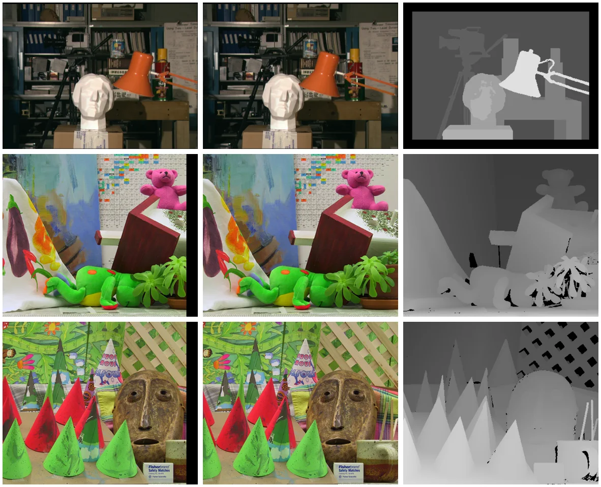
Figures 8 to 10 of the report: Tsukuba, Teddy and Cones. Reference image, second view, ground-truth disparity. Look at the second column against the first: everything shifts left, and the near things shift further. That shift is the depth. These are re-crops of my own report’s figures, not the original dataset files, which are not in the repository. Credit for the data: Middlebury / Scharstein & Szeliski.
For scoring, the recommended measure is the bad-N percentage: the fraction of pixels whose disparity is more than pixels from the truth. The report quotes the datasets’ recommended bad1, bad2 and bad4; the code computes 1, 2, 3 and 5. Border pixels are excluded, because a window cannot reach the edge of the image and so no valid disparity exists there.
Every knob, live
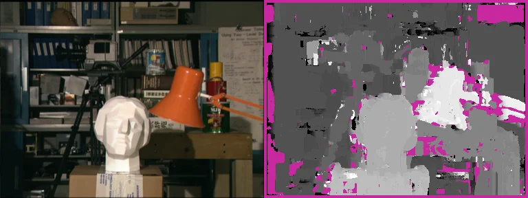
With JavaScript on, this becomes the matcher itself: choose SAD, SSD or ZNCC, drag the window size, the disparity bound and the accept threshold, change the exposure of one image, hover any pixel to see its cost curve, and download the result. It runs the Rust port in a worker, and reports the milliseconds each pass took.
Four things are worth doing with it before reading on.
Drag the accept threshold to zero and back. Everything the matcher is unsure about turns to the flag colour and then comes back. The widget flags a rejected match in whichever hot colour the theme uses, where the original wrote a black zero. That flag is not failure; it is the only way the algorithm has to admit it doesn’t know.
Turn the exposure of the right image down and watch SSD collapse. Then switch to ZNCC
and watch it not care. This is the entire argument of §4.2 in one slider. With the bundled
Tsukuba pair, right gain at and everything else at its default, the numbers
the widget prints go like this:
| matched | bad1 | |
|---|---|---|
| SSD, gain ×1 | 77.2 % | 31.7 % |
| SSD, gain ×0.7 | 19.5 % | 63.4 % |
| SAD, gain ×1 | 98.4 % | 36.4 % |
| SAD, gain ×0.7 | 75.5 % | 67.2 % |
| ZNCC, gain ×1 | 93.9 % | 34.3 % |
| ZNCC, gain ×0.7 | 93.4 % | 34.5 % |
SSD throws away three quarters of the pixels it used to accept, and of the ones it keeps, twice as many are wrong. SAD keeps more of them, which is worse, not better: its threshold is the more permissive of the two, so it accepts a great many matches that a brightness difference has already ruined. ZNCC does not move at all. That is what the normalisation is for, and it is the only thing in this post that behaves exactly as advertised.
Switch to the synthetic scene. It is generated inside the Rust crate from a disparity map I chose, so its ground truth is exact rather than measured: random dots on the background, a dotted panel at disparity 18, a flat grey panel at 12, and a striped panel at 22 whose bars repeat every 8 pixels. Everything that can go wrong with block matching is in one 384 × 288 image.
Hover a pixel. That is the part I would keep if I could keep only one.
Reading a cost curve
The cost curve is the plot of cost against disparity for a single pixel, the numbers the
argmin chose between. Once you can read one, most of the failures in a
disparity map stop being mysterious.
- A sharp V. A well-textured patch. One disparity fits and the others do not; the minimum is deep and narrow, and the answer is almost certainly right.
- A flat line. A textureless patch. On the synthetic scene’s grey panel the cost is identically zero at every disparity, because a flat window matches a flat window perfectly wherever you put it. SSD accepts it with complete confidence and reports the first disparity in the range; ZNCC’s is zero, its correlation is zero, and the threshold throws the pixel away. One of them knows that it does not know, and that is the best argument for ZNCC in this whole post.
- Several equal minima. Repeated texture. On the striped panel, whose bars repeat every 8 px and which sits at a true disparity of 22, the curve has identical minima at 6, 14 and 22. Ties go to the smallest disparity, so the matcher confidently answers 6 and the panel comes out at the wrong depth, cleanly and consistently. No threshold saves you here: the match is a perfect one, just not the right one.
- No good minimum anywhere. Occlusion. The band down the left of every raised object is visible in the left image and hidden behind that object in the right one, so the correct answer is not in the search range at all, it is not anywhere. The curve wanders, the best of a bad set wins, and the only defence is the threshold.
That is four distinct failure modes, all readable off one small plot, none of which the disparity map itself distinguishes from a correct answer.
The window is a bias–variance dial
The window half-width is the other knob that changes everything. It sets the amount of evidence behind each decision, and it does so at a cost that is exactly the classic trade-off.
Small windows have little to go on, so they are noisy, but they hug object boundaries, because the window stops seeing across an edge sooner. Large windows are far more reliable in flat and repetitive regions, but they fatten objects: any window straddling a depth discontinuity is dominated by whichever side has more texture, and the near surface bleeds outward by roughly pixels. Slide from 1 to 9 on the Tsukuba pair and watch the head grow a halo while the speckle disappears. There is no setting that gets both.
The default in the code is W=4, a window: 243 samples per comparison on a
colour image.
Rewriting it in Rust
The reason this post has a live widget and the 2019 version had a directory of PNGs is arithmetic. A single SSD pass over Tsukuba at 32 disparities, summed the obvious way, is
multiply-accumulates. That is not a slider-drag number in any language, and the NumPy version is worse than the count suggests because it re-reads the whole materialised window array once per disparity.
The port lives in a small Rust crate compiled to WebAssembly, and it differs from the NumPy in four ways that are worth being explicit about.
It aggregates instead of summing. For each disparity, the Rust builds one per-pixel
term image (, , or the product ) and then box-sums it with
separable running sums, two additions per pixel per pass. The window size drops out of the
inner loop entirely: a window costs the same as a one. That
turns operations into about , and it is exact rather than
approximate, because everything is an integer sum of u8 terms.
It expands ZNCC rather than pre-normalising it. The NumPy’s trick, normalise every window up front so the correlation becomes a dot product, is the right move in NumPy and impossible here: the normalised window stack is floats, which at is over four hundred megabytes. Expanding the product instead,
needs only a mean and a per pixel, both of which are box sums of and , and gives the same number. It is the more expensive of the two paths: three box sums per disparity instead of one, because the normalisation is per channel, and that shows up in the timings below.
It marks the borders invalid instead of shrinking the image. The Python’s output is
, which is why the evaluation has to slice
[30:-30] against [34:-34] to line the two up. The Rust keeps the image size and sets a
validity flag, so nothing silently shifts by . It also refuses to report a pixel whose
search would run off the left edge, where the Python’s clamped slice quietly searches a
shorter range instead.
Its thresholds are per-sample. thresh is mean for SAD, RMS for
SSD and correlation for ZNCC, so the number means the same thing at every window size. The
defaults are the originals converted: 25.5 for SAD (the report’s divided
by ), 9.2 for SSD (, from the code’s constant), and 0.6 for ZNCC (the
report’s number, not the code’s 0.1).
The crate is 26.8 kB of WebAssembly with no dependencies, and it runs the matcher in a
worker so a slider drag never blocks the page. On this laptop, one pass over the bundled
384 × 288 pair at and 32 disparities costs about 40 ms for SAD or SSD and 115 ms
for ZNCC outside the browser, and nearer 65 and 135 ms inside it; the widget prints the
number it measured on yours. Building the crate at opt-level = 3 rather than the
workspace’s "s" made it consistently slower (63 ms and 218 ms) and 12 kB larger, which
was not the result I expected and is the reason there is no per-package profile for it. Seventeen tests hold it in place; four of
them are the ones I would write first if I did this again:
- a synthetic pair at a known constant shift comes back with exactly that disparity at every valid pixel, for all three cost functions;
- a gain of and a lift of 30 grey levels on one image leaves ZNCC’s disparities untouched and its correlation above 0.99, while SSD (at the threshold the code’s own constant implies) accepts not one pixel of the 4060 in the test region; undoing the gain makes SSD perfect again, so it is the photometry that broke it and not the texture;
- the cost curve, computed the slow direct way, has its argmin at exactly the disparity the fast box-aggregated pass reported, and the same value there;
- nothing within a window of an edge, and nothing whose search would leave the image, is ever reported as a match.
What I would do differently
Three things, in order of how much they would improve the pictures.
Sub-pixel disparity. The whole matcher reports integers. Fitting a parabola to the cost at the argmin and its two neighbours costs three multiplications per pixel and typically halves the error; on a curve you can already see plotted, it is close to free.
A left-right consistency check. Match left-to-right, match right-to-left, and keep only the pixels that agree. That finds occlusions properly instead of hoping a threshold catches them, and it is the single biggest quality win available to a block matcher.
A cost threshold that means something. “Accept if the cost is below a fifth, or a tenth, or 85 per sample, of the maximum” is a number pulled out of the air, and this post has already spent two callouts on how badly that went. The ratio between the best and the second-best disparity is a far better confidence measure: it is exactly what distinguishes the sharp V from the flat line and the repeated texture, it needs no scale, and the cost curve was sitting there the whole time.
The next post is about the other half of this work: what those bad-pixel percentages actually measure, and how a table can read as a catastrophe while the pictures look fine.