Blog · Features and preprocessing ·
Kernels: box, Gaussian, median, min/max, and deriving Sobel
Convolution is a weighted sum, and everything changes with the weights: from "average the neighbours" to "take the median instead" to "the weights are a derivative, so the output is an edge map", with a Rust/WASM bench you can point at your own camera.
- interactive
- convolution
- filtering
- median-filter
- sobel
- laplacian
- rust
- wasm
Section 5 of the image-processing report is four pages long and it contains, as far as I can tell, one idea. A kernel is a little table of numbers; you slide it over the image and each output pixel is the weighted sum of the neighbourhood under it. Change the numbers in the table and you get a blur, or an edge map, or a sharpening filter, or a second derivative. Change the operation from “weighted sum” to “sort them and take the middle one” and you get the filter that beats all of the above at the job they were supposed to be good at.
That last sentence is the whole post. Everything else is arithmetic.
A kernel is a weighted sum
The report defines it in one equation. A kernel is an odd-shaped matrix: the report uses , indexed from to , so the centre tap has index and every kernel has a well-defined middle. Then:
That is Eq 5.1, and it is worth staring at for a second, because it is not quite convolution. A convolution flips the kernel before it slides (), and Eq 5.1 does not. What it defines is correlation. For every symmetric kernel in this post (the box, the Gaussian, both Laplacians) the two are identical and nobody has ever been harmed by the confusion. For the Sobel operator, which is antisymmetric, the flip is exactly a sign change, and that turns out to be the source of a real discrepancy between the report’s equations and the figures it printed. I get to that at the end.
The simplest weights there are
Set every weight to the same number and normalise so they sum to one. That is Eq 5.2, the box:
The implementation is one line:
def uniform_neighborhood_averaging(src, kernel_size=3):
return cv2.filter2D(src, -1, np.ones((kernel_size, kernel_size)) / (kernel_size * kernel_size))The driver script that produced the report’s figures runs it at on a kidney angiogram to make Figure 16:
fig0235_d_local_averaging_out = uniform_neighborhood_averaging(fig0235_c_kidney, 41)A box is a serious blur: each output pixel is the mean of 1 681 inputs, and it is the reason the next section exists.
Why a 41 × 41 box is not 1 681 multiplies
Written out as Eq 5.1, a kernel costs multiply-adds per pixel. At on a 640 × 480 frame that is half a billion taps, which is exactly the kind of number that makes people say “you can’t do that in a browser”.
You do not have to do it that way, for two reasons that stack.
A box separates. The all-ones matrix is the outer product of two all-ones vectors, so blurring across and then blurring down gives the same answer for taps instead of . That is a 20× saving at before you have been clever at all.
Within a pass, the window is a running sum. Moving the window one pixel to the right adds one sample and drops one. So the per-pixel cost of each pass is two additions, independent of entirely. The whole filter is per pixel at any radius. The Rust version of the running sum:
let mut sum: f64 = line[..k].iter().map(|&v| v as f64).sum();
let out = &mut tmp[y * w..(y + 1) * w];
out[0] = sum as f32;
for x in 1..w {
    sum += line[x + k - 1] as f64 - line[x - 1] as f64;
    out[x] = sum as f32;
}
The vertical pass is the same trick with a rolling accumulator per column, so it also never touches a pixel twice. A unit test asserts the two agree, comparing them at and requiring the worst pixel to differ by less than a hundredth of a grey level.
Timed natively on a 640 × 480 image, release build:
| box filter, | time |
|---|---|
| every tap (Eq 5.2 as written) | 1 307 ms |
| separable running sum | 1.26 ms |
A thousand times faster for the same output. The widget below runs the same comparison in your browser, on WebAssembly rather than native code, so you can see what the number is on your own machine.
Weighting by distance
If averaging the neighbours equally seems crude (the pixel two steps away gets the same vote as the one next door), the fix is to weight by distance. Eq 5.3:
The Gaussian wrapper:
def gaussian_filtering(src, kernel_size=3, sigma_x=0.0, sigma_y=0.0):
    return cv2.GaussianBlur(src, (kernel_size, kernel_size), sigmaX=sigma_x, sigmaY=sigma_y)
The default of 0.0 is not “no blur”: OpenCV reads a zero as “pick one to suit
the kernel size”, using , which gives 0.8 at
, 1.1 at and 6.5 at . My Rust does the same, so the widget’s
“auto” setting means the same thing as the Python’s.
The driver, though, passes an explicit of 0.4 at :
fig0335_a_pcb_noise_gauss_sxsy_0_4 = gaussian_filtering(fig0335_a_pcb_noise, 3, 0.4, 0.4)and that number explains something you can see in the figure below. A 1-D Gaussian with sampled at and normalised is . Applied along both axes, the centre tap keeps of its weight: 85 % of each output pixel is the input pixel. It is barely a filter. Whatever the Gaussian panel of Figure 17 shows, it is not what a Gaussian blur is capable of.
When the average is the wrong answer
The report then does the thing that makes the section worth reading. It takes a printed circuit board buried in salt-and-pepper noise and runs three filters at across it: the box, the Gaussian at , and the median.
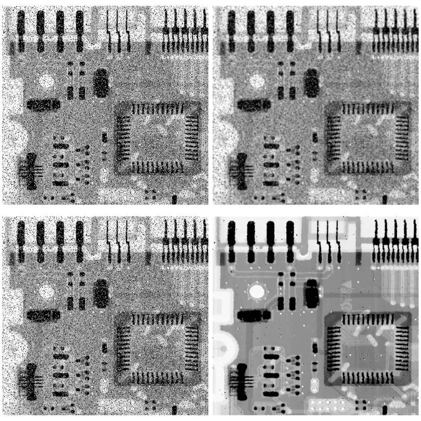
Figure 17 (p. 15), with the report’s sub-captions dropped: (top left) the noisy original, (top right) local averaging, (bottom left) the Gaussian at , (bottom right) the median. Original plate from Gonzalez & Woods, Digital Image Processing 3E.
The bottom-right panel is the point of the whole section. The box turned the speckle into a grey mottle: it spread every bad pixel over its nine neighbours instead of removing it. The Gaussian at barely touched it, for the reason computed above. The median deleted it, and left the traces sharp while doing so.
The arithmetic behind that is embarrassingly simple. Take nine pixels of a flat grey region where one has been flipped to 255. The mean moves by levels: the outlier is shared out, not removed, and it contaminates all nine outputs as the window passes over it. The median does not move at all, because the middle of the sorted list is still one of the eight good values. A linear filter has to give the corrupt sample some weight; a rank filter can give it none.
The report’s own summary of it, from page 15, is more measured than mine:
Figure 17 shows how [Gaussian] blur and local averaging filters can be used for noise reduction in an image before the image is processed. However, for regions with point noise, they are not as good as the median filter.
Min and max are the same family: sort the neighbourhood and take the first or the last.
min_filtering and max_filtering reach for cv2.erode and cv2.dilate,
which on a grey-scale image with a rectangular structuring element are exactly the local
minimum and the local maximum:
def min_filtering(src, kernel_size=3):
    return cv2.erode(src, cv2.getStructuringElement(cv2.MORPH_RECT, (kernel_size, kernel_size)))
On text they do the obvious violent thing, which is Figure 18:

Figure 18 (p. 15): the original plate, then a max filter, then a min filter. Bright text on a dark ground, so max fattens the glyphs and min eats them. Plate from Gonzalez & Woods, DIP3E.
For bright-on-dark text, max is dilation of the strokes and min is erosion of them. Swap the polarity (dark ink on white paper, which is what everything you actually scan looks like) and the two exchange roles. The report notes that the two are “often used together to reduce noise”, which is the opening–closing pair: a min followed by a max removes bright specks and puts the shapes back roughly where they were.
Break it, then fix it
Here is the section as a thing you can drive. It starts on the report’s own noisy PCB with a box (Figure 17(b)) and the buttons walk the argument:
- Break it buries the picture in Gaussian noise and 8 % salt and pepper, and puts the box filter on it. Watch the speckle turn to mottle.
- Fix it (median) switches the one control that matters. Nothing else changes.
Then keep going. Drag the kernel size to 41 and feel the difference between the box (which does not care) and the median (which cares a little). Switch to Text and try min and max. Switch to Bone scan and try the derivative filters from the next section. Point it at your camera, or drop in a photo of your own. Nothing is uploaded anywhere; the frames go straight to the WebAssembly module in this tab.
With JavaScript on, this becomes a live filter bench: pick a picture (or your camera), add Gaussian and salt-and-pepper noise, choose between box, Gaussian, median, min, max, Sobel, the two Laplacians or a kernel you type yourself, drag a divider to compare against the input, and download the pair as a PNG.
The Custom… filter is the one to spend time in. Every kernel in this post is a preset button under it, including the two that the report and OpenCV disagree about, so you can load them side by side and see the disagreement rather than take my word for it.
One routine for min, median and max
There is a reason the median is not the filter people reach for first, and it is that the obvious implementation is terrible. Sorting values per pixel is per pixel; at on a 640 × 480 frame that is 2.7 seconds in optimised native code. The naive box was bad; the naive median is worse.
Huang’s algorithm fixes it the same way the running sum fixed the box: by noticing that consecutive windows share almost all their pixels. Keep a 256-bin histogram of the window instead of a sorted list. Sliding one pixel right means removing the pixels of the column that left and adding the of the column that arrived: histogram updates instead of comparisons. Then keep a cursor on the histogram: the current answer, and the number of samples strictly below it.
for each row:
    build the histogram of the k×k window at x = 0
    cursor ← (value 0, count-below 0)
    for each x:
        if x > 0:
            for each of the k rows of the window:
                hist[leaving pixel] −= 1 ; if it was below the cursor, count-below −= 1
                hist[entering pixel] += 1 ; if it is below the cursor, count-below += 1
        while count-below > rank:            # the cursor is too high
            cursor −= 1 ; count-below −= hist[cursor]
        while count-below + hist[cursor] ≤ rank:   # the cursor is too low
            count-below += hist[cursor] ; cursor += 1
        output ← cursor
The two while loops usually run zero or one times, because one column of pixels
cannot move the rank very far. The cost per pixel stops depending on and starts
depending on .
The nice part is what falls out for free. Nothing in that loop knows what a median is: it finds the value at a given rank. Rank 0 is the minimum, is the maximum, and is the median, so one routine serves all three filters of the previous section. That is the whole export:
/// `rank` 0 is the minimum, `k²/2` the median and `k²−1` the maximum:
/// three filters, one routine, one histogram.
#[no_mangle]
pub extern "C" fn apply_rank(ptr: *mut u8, w: usize, h: usize, k: usize, rank: usize)
Two unit tests keep it correct: one checks ranks 0, and against a brute-force minimum, median and maximum, and another checks six different ranks at against a sort. They have to agree pixel for pixel, not approximately.
| median filter, 640 × 480 | sorting | histogram | speed-up |
|---|---|---|---|
| 394 ms | 14.6 ms | 27× | |
| 2 735 ms | 17.3 ms | 158× |
Look at the middle column rather than the ratio. Going from to costs the sorting version seven times more work and the histogram version 18 %. That flatness is what makes the kernel-size slider in the widget usable all the way to 41.
Weights that differentiate
Everything so far has been a smoothing filter. The second half of section 5 changes what the numbers in the table are for.
An edge is a place where intensity changes sharply, so an edge is a large gradient, so if you can approximate a derivative with a kernel you have an edge detector. The crudest approximation is the forward difference, Eq 5.4:
Note where the derivative lives: at , half a pixel to the right of any pixel you have. A difference of two samples estimates the slope between them. That half-pixel offset is a real problem: every edge you find is displaced by half a pixel in the direction you differenced.
The fix is to average the forward difference with the backward one, which lands the estimate back on the pixel. Eq 5.5, the central difference:
As a kernel that is : the centre pixel is not used at all, which is a slightly startling property for a derivative estimate and is why a central difference is blind to a one-pixel spike.
Now the last step, and it is the one the report states rather than derives, so let me derive it. A single row of is a fine derivative and a terrible one: it is a three-tap filter with no averaging in it, so a single noisy pixel produces a full-strength edge. Take the same difference on the row above and the row below as well, and add the three up with the middle one counted twice: that is a smoothing down the column, the binomial approximation to a Gaussian. Multiply the two out:
and that is Eq 5.6:
Sobel is not a magic edge kernel. It is a central difference along one axis and a binomial blur along the other, in that order, and because it is an outer product it separates: the Rust applies it as two 3-tap passes, reusing the same separable-convolution routine the Gaussian uses. The report puts it the same way, that it “combines both a Gaussian blur with a gradient operation”, which is right if you accept as a Gaussian; it is the third row of Pascal’s triangle, and the binomial coefficients converge on a Gaussian as the row gets longer.
The second derivative
If the first derivative peaks at an edge, the second derivative crosses zero at one, which is a sharper localisation and a much noisier one. Eq 5.7 is the Laplacian:
Apply the central difference twice along each axis and you get per axis; add the two axes and the centre taps sum to . That is Eq 5.8:
It only looks along the axes, so it responds differently to a diagonal edge than to a horizontal one. Including the diagonal neighbours (with the centre now at , so the weights still sum to zero and a flat region still gives zero) makes it very nearly isotropic. Eq 5.9:
Both are in the widget, and the difference between them on a curved edge is visible if you load the bone scan and flip between them.
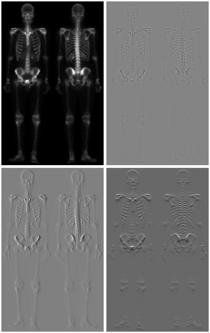
Figure 19 (p. 17): (top left) the original bone scan, (top right) the Laplacian, (bottom left) Sobel , (bottom right) Sobel . The two Sobel panels are the same operator turned ninety degrees: look at the ribs, which are nearly invisible in one and the strongest thing in the frame in the other. Plate from Gonzalez & Woods, DIP3E.
The embossed look of the two Sobel panels is not a stylistic choice; it is what a signed
image looks like when you display it with matplotlib’s default scaling. The gradients run
from strongly negative to strongly positive, zero lands in the middle of the grey ramp, and
an edge lit from one side comes out bright while the same edge on the other side of the
bone comes out dark. The Python operators module’s own commented-out demo displays them
through cv2.convertScaleAbs instead, which takes the absolute value and loses the
direction. The widget offers both, plus the raw clip, under “show as”: it is worth flipping
between them
on the Sobel filters, because “auto-scale” and “absolute value” tell you genuinely different
things about the same array.
There is one more thing Figure 19 shows without saying it. The Laplacian panel is almost entirely flat grey with a thin, speckled outline, while the two Sobel panels are legible images. That is the smoothing column doing its work: Sobel has a blur built into it and the Laplacian has no smoothing anywhere, so the second derivative amplifies exactly what you do not want. Turn the noise up in the widget with the Laplacian selected and it disappears into static long before Sobel does, which is the same conclusion the edge-detector benchmark reached by counting, on a synthetic image, a few weeks earlier.
Where the pictures came from
What I would do differently
Two things, mostly.
The Gaussian in Figure 17 is not a fair comparison. At it keeps 85 % of each pixel, so the panel shows a filter that was barely switched on losing to a filter that was. A fair one tunes the box, the Gaussian and the median until they smooth a clean region by the same amount, then asks which still has edges left. The median would still win on salt and pepper, by a smaller and more interesting margin.
And I would have checked what cv2.Laplacian(ksize=3) actually convolves with before
printing two Laplacian kernels next to a figure made by a third. That one is not a matter of
taste; the report says something that is not true of its own figure, and it took a
reimplementation eighteen months later to catch it. Reimplementing something you have
already written up is an oddly effective form of proofreading.