Blog · Features and preprocessing ·
Which edge detector survives noise?
A Monte-Carlo benchmark of Canny, Sobel and the Laplacian on a synthetic step edge buried in Gaussian noise (30 000 trials, two curves, one surprise), rebuilt in Rust so it runs in your browser.
- interactive
- edge-detection
- canny
- sobel
- laplacian
- monte-carlo
- rust
- wasm
Everyone who has used OpenCV has an opinion about Canny versus Sobel. Almost nobody has a number. The trouble is that you cannot score an edge detector on a photograph, because a photograph has no ground truth: where the edge “really” is depends on who you ask. This was the first experiment in a report I wrote up at the time comparing feature detectors and descriptors, and I did the only thing that would actually let me score it: I built an image where I knew where the edge was, buried it in progressively worse noise, and counted.
The whole experiment lives in one self-contained Python script. It needs no dataset, it synthesises everything, and it produced the two figures I still think are the most interesting measurement in the whole project. It also produced one curve that goes the wrong way, which is the part worth reading for.
The protocol
The report sets it out in six steps, which I will paraphrase:
- Make a test image with two regions split down the middle, each filled with samples from a Gaussian with a different mean.
- Run the edge detectors on it and compare their output to the theoretical optimal edge: the split.
- Count the true-positive and false-positive pixels.
- Average over many runs.
- Tie the noise and the contrast to a single knob: the noise has standard deviation and the two means are and .
- Repeat for a range of .
Step 5 is the trick that makes the whole thing a one-parameter problem. As grows the noise gets worse and the two regions slide toward each other, so the contrast-to-noise ratio falls monotonically. At the image is a perfect 255-to-0 step; at the halves are centred on 135 and 120 with a standard deviation of 120, which is barely an edge at all.
Building a ground truth
The image is 100 × 100. The ground truth is two columns wide, because a step between column 49 and column 50 can reasonably be reported on either side of it. Here is the code that builds it:
edge_mask = np.zeros((100, 100))
edge_mask[:, 49:51] = 1

noisy_image = np.clip(np.random.normal(sigma, sigma, edge_mask.shape), 0, 255).astype(np.uint8)
noisy_image[:, :50] = np.clip(np.random.normal(255-sigma, sigma, (100, 50)), 0, 255).astype(np.uint8)
Every pixel is drawn from , then the left fifty columns are overwritten
with . The clip and the astype matter more than they look: a
sample is clamped to and then truncated to an integer, so at large a
lot of the bright half piles up at exactly 255 and the dark half at exactly 0. The
detectors see that distribution, not a clean Gaussian.
Three detectors, three fixed thresholds
Each trial runs three detectors on the same noisy image:
edges_c = cv2.Canny(noisy_image, 40000, 55000, apertureSize=7, L2gradient=False)

edges_l = np.abs(cv2.Laplacian(noisy_image, cv2.CV_64F)) > 230

edges_s = (cv2.Sobel(noisy_image, cv2.CV_64F, 1, 0, ksize=7) ** 2 + cv2.Sobel(noisy_image, cv2.CV_64F, 0, 1,
                                                                          ksize=7) ** 2) > 6658560000
These are OpenCV’s detectors, not mine; the work here is the benchmark around them. The thresholds were picked once, by hand, so that each detector reported exactly the two mask columns on the clean image, and then held fixed for the whole sweep. That is the fairest thing I could think of at the time, and it is also the experiment’s biggest weakness: the curves below are the curves for these thresholds. Further down the page, the sweep widget lets you move the thresholds yourself and watch the ranking argue back.
The numbers look arbitrary but are not. OpenCV’s 7-tap Sobel is the separable pair
and . On a clean 255-to-0 step the
horizontal derivative in the two mask columns is , and in the
columns either side of them it is exactly half that, . The Sobel threshold,
, is ; with a strict >, the neighbouring columns sit on the
threshold and are excluded, so the clean image scores 100 % TP and 0 % FP. The Laplacian
(OpenCV’s default 3 × 3 kernel, ksize=1) gives in the mask columns and zero
elsewhere, so > 230 does the same job. The Canny thresholds are on the same 7-tap
gradient scale, using the L1 magnitude .
Scoring: rows for TP, pixels for FP
This is the detail that makes the numbers interpretable. Here is the scoring code, repeated for each detector, and the normalisation that follows it:
edges_in_mask = edges_c*edge_mask
correct_count_canny[j, i] = np.count_nonzero(np.sum(edges_in_mask, axis=1))
incorrect_count_canny[j, i] = np.count_nonzero(edges_c) - np.count_nonzero(edges_c*edge_mask)

total_correct_in_mask = np.count_nonzero(np.sum(edge_mask, axis=1))
total_incorrect_in_mask = np.count_nonzero(edge_mask == 0)
avg_corr_canny = np.average(100*correct_count_canny/total_correct_in_mask, axis=1)
avg_incorr_canny = np.average(100*incorrect_count_canny/total_incorrect_in_mask, axis=1)
A true positive is a row that contains at least one detection inside the two-column mask, out of 100 rows. So a wobbly edge that lands on column 49 in some rows and 50 in others still scores 100 %, and a detector that finds the edge in every row but paints both mask columns gets no extra credit. A false positive is any detected pixel outside the mask, out of the 9 800 pixels that are not in it. The two rates therefore have different denominators, which is why the FP axis tops out at 63 % while that number means “two thirds of the image was called an edge”.
The sweep is np.linspace(0, 120, 100), a hundred values of , 300 trials each,
three detectors: 30 000 synthetic images and 90 000 edge maps, or about 900 million
pixel-detector evaluations. It took the Python minutes to run.
The results
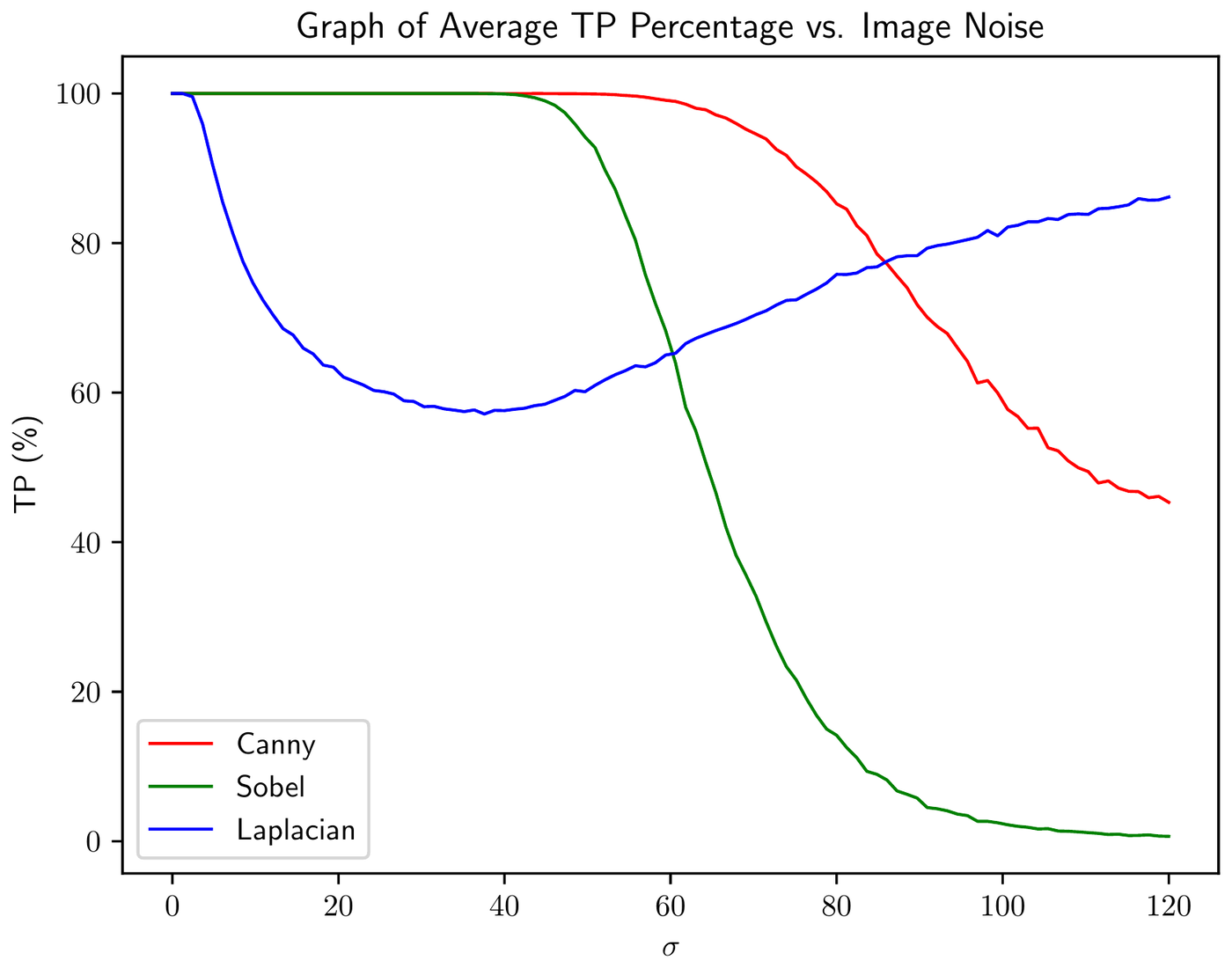
Figure 32 from the report (p. 35): average TP percentage against , 300 trials per point.
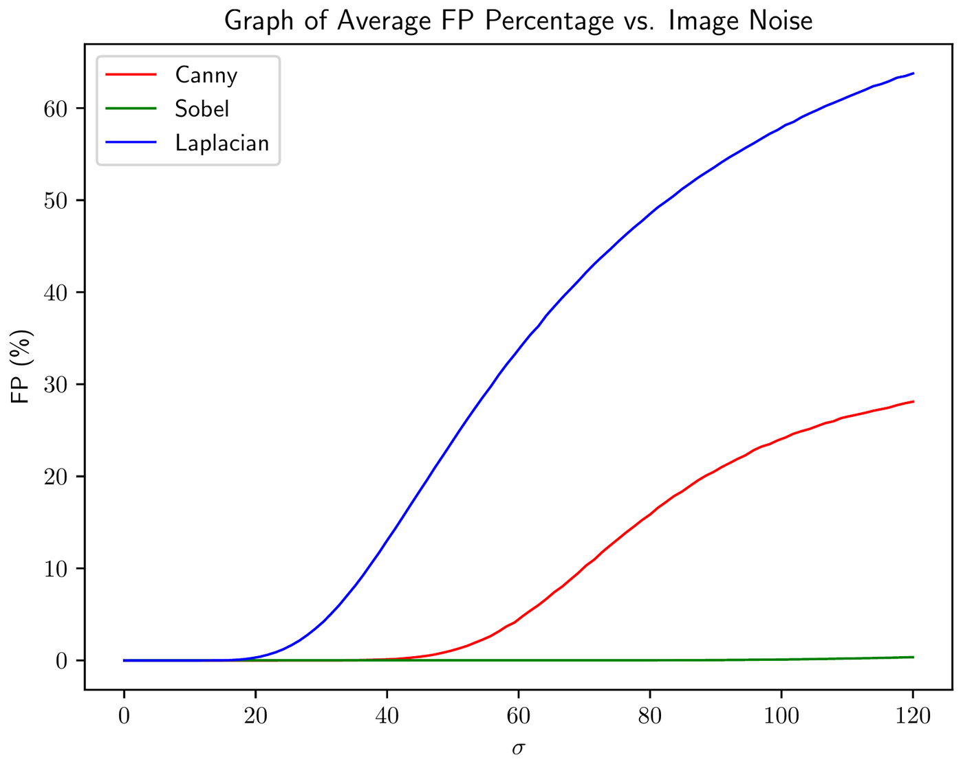
Figure 33 (p. 35): average FP percentage against . Read it together with the plot above. Neither means anything alone.
The two plots have to be read as a pair, and the pair says something different about each detector. Reading them off the figures:
Sobel, with this threshold, is a detector that would rather say nothing than be wrong. The 7-tap kernel averages over a 7 × 7 window, and the threshold is half the clean response, so noise alone almost never reaches it. But once the contrast has dropped far enough that the edge itself no longer reaches it, the detector simply goes quiet. Canny is the opposite temperament: hysteresis lets a strong seed drag its weaker neighbours along, so the edge keeps being traced long after Sobel has lost it, and for the same reason the detector starts tracing contours through the noise as well.
The Laplacian’s curve goes the wrong way
The blue curve in Figure 32 is the one I keep coming back to. A detector’s true-positive rate is supposed to fall as noise increases. The Laplacian’s falls, and then it recovers, and by it is scoring better than Canny.
It is not getting better. The 3 × 3 Laplacian is a second-derivative operator with no smoothing at all, so it is the most noise-sensitive of the three by construction; its TP rate collapses first for exactly that reason. But look at the FP plot: by the time the TP curve turns around, the Laplacian is calling 20 %, then 40 %, then 63 % of the image an edge. When two thirds of the pixels are “edges”, the probability that at least one of the two mask pixels in a given row is among them is high, and that is all a true positive requires. The curve rises because the detector is firing everywhere and the edge is being included by accident.
This is the lesson of the experiment in one curve: a true-positive rate quoted on its own is meaningless. Any detector can reach 100 % TP by returning a white image. The Laplacian did a softer version of that, and a single-number benchmark would have rewarded it.
What the edge maps look like
The report also kept the first trial at four values of , which are worth seeing next to the curves.
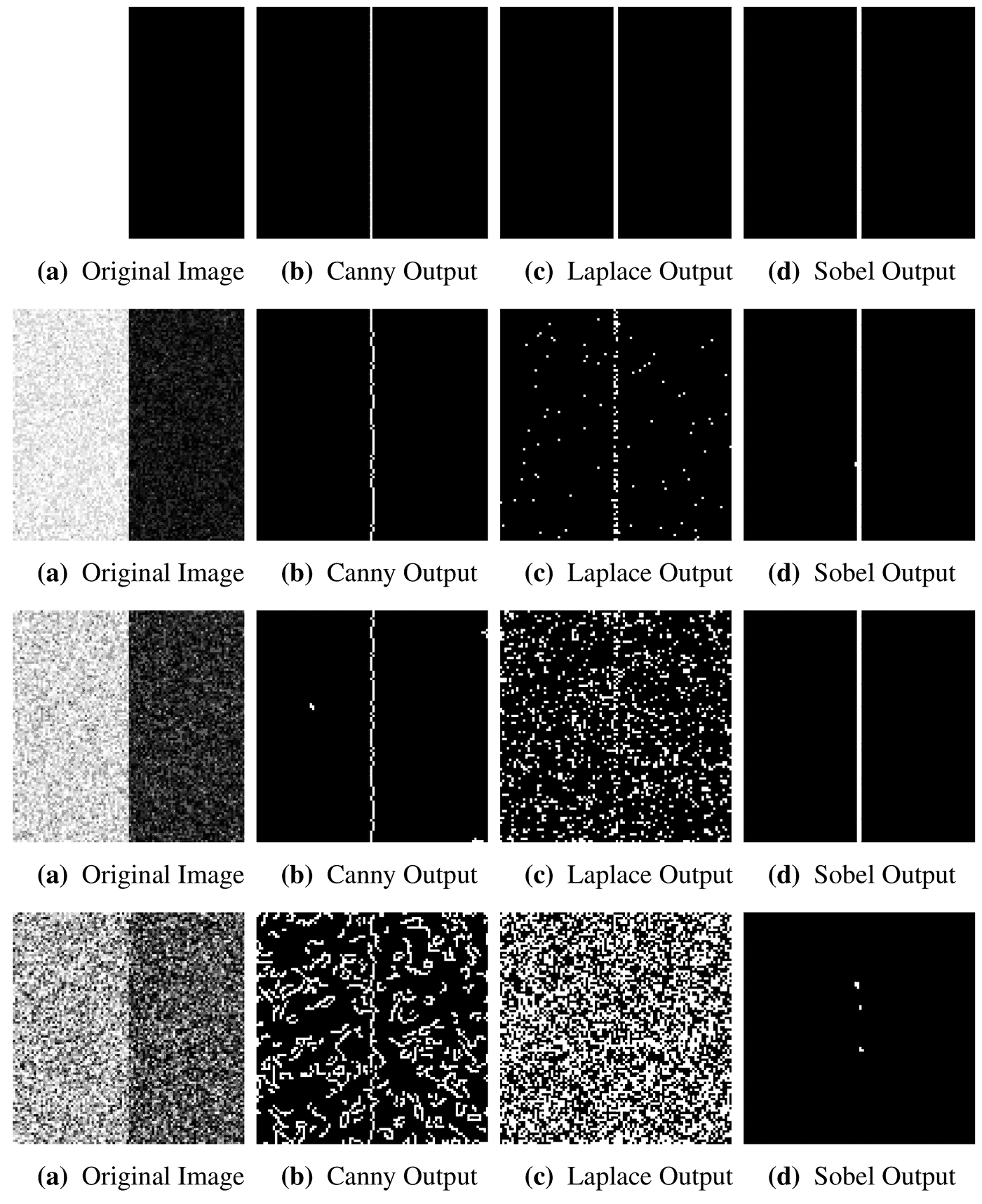
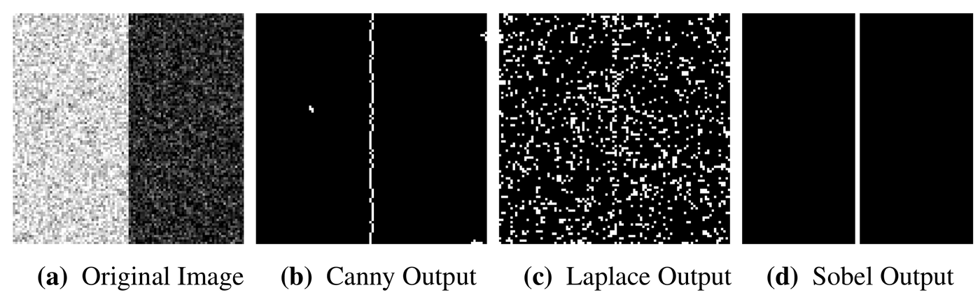
Figures 34–37 (p. 36): the first trial at = 0, 21.82, 40.0 and 80.0: original, Canny, Laplace, Sobel.
At the Laplacian panel is visually pure noise, while its TP number on the curve is a respectable-looking 58 %. At Canny is still drawing one clean vertical line down the middle (you can see it) but it is also drawing a great many short contours through the noise, and the Sobel panel has gone almost entirely dark with a few dots near the centre. Every claim in the two plots is visible in these sixteen tiles.
The report’s discussion (§8.3, p. 48) put it this way:
The edge detectors are very resilient to additions in noise, with the Sobel detector managing to retain the lowest false positive rate. However, the Canny edge detector was able to obtain a large true positive rate even when the image contained large amounts of noise. Furthermore, the false positives which it identified, were fairly just as the noise levels in the image created quite a few edges.
“Fairly just” is doing a lot of work in that last sentence, but I stand by it: look at the input and there really are edges in the noise.
Try one trial
The Python ran on a laptop and printed percentages. To put the experiment on this page I
rewrote it in Rust and compiled it to WebAssembly, the imaging-wasm crate, which several
later posts share. Below is one trial. Drag , reroll the noise, and watch the
per-trial TP and FP counts jump around; that jumpiness is why 300 trials per point were
necessary. Detections inside the two mask columns are drawn in the accent colour, everything
else in ink, and the mask itself is the faint band.
With JavaScript on, this becomes a live trial: a σ slider, a reroll button, the four images and the per-trial TP/FP counts.
The seed is shown so a trial can be shared: the same seed and produce the same
image on every machine, because the noise comes from a PCG32 generator seeded from that
number rather than from np.random. The thresholds are live too: lower the Sobel
threshold and it starts behaving like the Laplacian; raise Canny’s low threshold and
hysteresis loses its weak links.
Run the benchmark yourself
This is the part no static figure can show. Press Run and the sweep happens in your browser: every gets a couple of trials first, so a rough, jittery version of both curves appears within a second, and then each further pass thickens the estimate until the noise settles into the shapes of Figures 32 and 33. Watching that convergence is the Monte-Carlo lesson.
With JavaScript on, this runs the Monte-Carlo sweep in a Web Worker and draws both curves as the trials accumulate.
The default is 60 trials per rather than 300, so a run takes about eight seconds on my laptop; the slider goes up to the report’s 300 if you want the full protocol, which takes around forty. The three thresholds are sliders, because the ranking is a function of them and I would rather you saw that than took my word for the curves. Try the Sobel threshold at 40 k and the Canny pair at 20 k/30 k.
Try it on your own picture
Everything above is a 100 × 100 synthetic step, because that is the only image whose edges I could score. But the detectors do not know that, and the same three kernels will run on anything, so the last island points them at whatever you give it, with the σ slider still wired to the benchmark’s noise model. Start with the bundled scene, then drag σ up and watch the three of them come apart in exactly the order Figures 32 and 33 predict: Sobel goes quiet, the Laplacian fills the frame, Canny keeps drawing contours, some of them the right ones.
Three things worth doing. Draw a thick stroke and turn σ up. Ink on white paper is a 255-level step (the benchmark’s own stimulus, drawn by hand), so the stroke itself is remarkably hard to lose: at the island’s default thresholds all three detectors still marked mine at σ = 100, though by then two of them were marking nearly everything else as well. The blank paper around the stroke is the thing to watch, and it goes in the order of Figure 33: the Laplacian is speckling it before σ = 10, Canny by σ = 40, while Sobel is still almost clean at σ = 60.
Switch to the test card, where the wide band beside the black step is a smooth ramp: a strong gradient with no step anywhere in it, which is exactly what an edge detector is supposed to ignore. At σ = 0 all three ignore it completely. By σ = 10 the Laplacian has called 37 % of that band an edge; Canny gets to 35 % by σ = 40; Sobel is still at 1 %. Those are the same three curves as Figures 32 and 33, on an image that did not exist until you pressed a button. And if you have a camera, hold a printed page up to it: text is the hardest thing in this post to keep, and you can find the σ at which each detector stops being able to read.
No image leaves your browser. The file you pick, the frame from your camera and the scribble you draw are handed straight to the WebAssembly kernels running in this tab; nothing is uploaded, stored or sent anywhere, and closing the page discards all of it. The camera only starts when you press the button and its track is stopped when you press it again or navigate away.
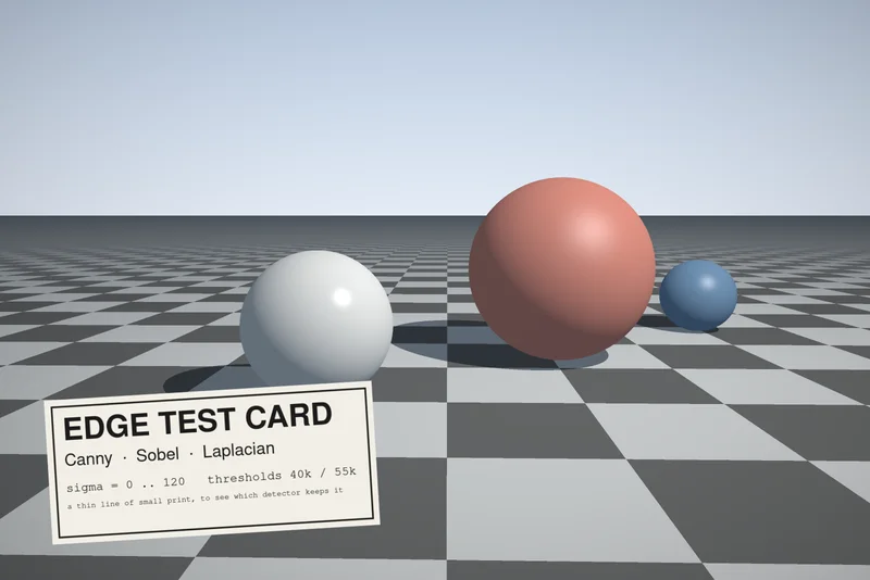
With JavaScript on, this becomes a live edge detector: pick the bundled scene, a synthetic test card, an upload, a scribble or your camera, choose Canny, Sobel, the Laplacian or all three, bury the picture in noise with the σ slider, and download the edge map.
The thresholds start about four times lower than the benchmark’s, and it is worth knowing why. The 7-tap Sobel answers a step of height with , so the report’s is a step of 128 grey levels, half the full range. Almost nothing in a photograph is that steep; the sharpest boundary in the sample scene is the silhouette against the sky, and even that is softened by the anti-aliasing. The live island therefore starts at , about 50 grey levels, and you can drag it back up to the report’s number to watch a real image go blank.
Reimplementing Canny
Sobel and the thresholded Laplacian are a convolution and a comparison. Canny is the only
real work, because there is no OpenCV in the browser and I wanted the browser numbers to
mean the same thing as the report’s. cv2.Canny is four stages:
- Gradient. Sobel , with the requested aperture (7 here), replicated borders, and either the L1 magnitude or the L2 one.
- Non-maximum suppression. A pixel above the low threshold survives only if its magnitude beats its two neighbours along the gradient direction. OpenCV quantises the direction into three cases using and : near-horizontal gradients compare left and right, near-vertical compare up and down, and everything else compares the diagonal pair chosen by the sign of .
- Double threshold. Survivors above
highare seeds; survivors aboveloware candidates. - Hysteresis. Flood from every seed through 8-connected candidates; whatever the flood reaches is an edge, the rest is discarded.
The suppression step is where an implementation quietly diverges from OpenCV, so I copied
its comparisons exactly, including the asymmetry of > on one side and >= on the other,
which decides which of two equal-magnitude columns wins on a perfect step. Here is the
comparison as I wrote it in Rust:
if ay < tg22x {
    keep = m > m_at(xi - 1, yi) && m >= m_at(xi + 1, yi);
} else {
    let tg67x = tg22x + (ax << (CANNY_SHIFT + 1));
    if ay > tg67x {
        keep = m > m_at(xi, yi - 1) && m >= m_at(xi, yi + 1);
    } else {
        let sgn: isize = if (xs ^ ys) < 0 { -1 } else { 1 };
        keep = m > m_at(xi - sgn, yi - 1) && m > m_at(xi + sgn, yi + 1);
    }
}
On the clean step, is 163 200 in both mask columns and 81 600 on either side of
them; the >= lets column 49 beat its equal neighbour, column 50 loses to it, and Canny
reports a single one-pixel line, which is exactly what the Canny panel of the
row above shows. A test pins that down: at the Rust Canny returns column 49 and
nothing else, and all three detectors score 100 % TP, 0 % FP.
What I would do differently
The thresholds. Fixing them so that the clean image scores perfectly is defensible, but it means the sweep compares three particular operating points, not three detectors. The better experiment sweeps each detector’s threshold at every and reports the whole precision–recall curve, or at least picks the threshold that equalises the FP rate across detectors. The widget above is a small step toward that: it will not draw the curve for you, but it will let you move the operating point and watch the ranking change, which is more than the report did.
And I would report the Laplacian’s TP curve with its FP curve stapled to it, every time. It is the best illustration I have of why one number is never enough.