Backprop from first principles (no autograd, no frameworks)

The second EAI732 assignment starts with a sentence that sounds like a formality and isn’t: construct a basic fully connected feed-forward neural network from first principles, then develop the backward propagation algorithm for it. From first principles means no autograd. It means you write down the error, differentiate it with respect to one weight buried inside two nested sums, and keep track of which index survives.

I wrote seven pages of derivation for that, and it is the part of the 349-page report I am still happy with, not because the maths is hard, but because I made myself do the index-juggling step in the open. Every textbook I read at the time wrote ”$\partial E / \partial w_{i,j} = \delta_j Z_i$, and by the chain rule the hidden layers follow similarly”. Similarly is doing a lot of work in that sentence. This post is the derivation with nothing skipped, the twelve lines of NumPy it turns into, and a sandbox where you can drop points on a square and watch the boundary bend around them.

One neuron

The whole model is one line. Writing $m$ for the layer, $i$ for the input index and $j$ for the output index:

$$Z^{(m)}_j = \sigma\!\left( \sum_{i=0}^{I} w^{(m)}_{i,j} Z^{(m-1)}_i \right)$$

The superscript $(m)$ is in brackets throughout to insist that it is a layer label and not a power. And the sum runs to $I$ inclusive, where $Z^{(m-1)}_I$ is fixed at 1: the bias. Making the bias an input pinned at unity rather than a separate additive term is a notational trick that buys a real thing: it gives the neuron a fixed point to adapt around, instead of forcing every parameter to be defined only relative to the others. Networks with it are, in my experience then and since, both more accurate and faster to train.

A network of them

Stack the neurons of a layer and the sum becomes a matrix product:

$$Z^{(m)} = \sigma\!\left( W^{(m)} \cdot Z^{(m-1)} \right)$$

with $\sigma$ applied element-wise, and the weight matrix laid out so that its row index is the output neuron and its column index is the input neuron:

$$W^{(m)} = \begin{bmatrix} w^{(m)}_{0,0} & w^{(m)}_{1,0} & \cdots & w^{(m)}_{I,0} \\ w^{(m)}_{0,1} & w^{(m)}_{1,1} & \cdots & w^{(m)}_{I,1} \\ \vdots & \vdots & \ddots & \vdots \\ w^{(m)}_{0,J} & w^{(m)}_{1,J} & \cdots & w^{(m)}_{I,J} \end{bmatrix}$$

That transposed-looking layout is not an accident and it is worth holding on to, because it is what puts a transpose in the backward pass. Forward propagation is then: set $Z^{(0)}$ to the input and apply the formula until you run out of layers.

procedure FORWARD-PROPAGATION(inputVector)
    Layers ← an M-element array holding W(m) for each layer
    outputVector ← inputVector
    for m from 1 to M do
        outputVector ← σ( Layers[m].W · outputVector + Layers[m].b )
    end for
    return outputVector
end procedure

Choosing the activation function

The activation function has to earn its place. The simplest choice is no activation function at all, which is useless the moment you stack layers: a composition of linear maps is linear, so a ten-layer linear network can represent exactly what a one-layer linear network can.

For classification the obvious next thought is a step function, and the obvious problem is that its derivative is a singularity in the one place you care about. So: the sigmoid, which is a smoothed step,

$$\sigma(x) = \frac{1}{1 + e^{-x}}$$

Those four properties are exactly the hypotheses of the universal approximation theorem, which is the licence to believe that a wide enough network can approximate any function to arbitrary accuracy. The other reason to like it is that its derivative is free:

$$\begin{aligned} \frac{\partial}{\partial x}\sigma(x) &= \frac{\partial}{\partial x}\frac{1}{1+e^{-x}} \\[4pt] &= \frac{\frac{\partial}{\partial x}(1) \cdot (1+e^{-x}) - \frac{\partial}{\partial x}(1+e^{-x})}{(1+e^{-x})^2} \\[4pt] &= \frac{e^{-x} + 1 - 1}{(1+e^{-x})^2} \\[4pt] &= \frac{1+e^{-x}}{(1+e^{-x})^2} - \left(\frac{1}{1+e^{-x}}\right)^{2} \\[4pt] &= \sigma(x)\bigl(1 - \sigma(x)\bigr) \end{aligned}$$

The derivative is a function of the output, not the input. Forward propagation already computed and stored $Z = \sigma(p)$, so the backward pass gets $\sigma'$ for one multiply and one subtract, with no exponentials and nothing extra to remember. That single fact is why the code below has no separate cache of pre-activations.

Two functions I considered and dropped. tanh is the same curve rescaled, $\tanh(x) = 2\sigma(2x) - 1$, so the choice between them is a choice of output range, and a sigmoid output in $(0,1)$ reads directly as a likelihood, which is more convenient. Softmax is genuinely useful for one-hot classification, but you can get most of the way by taking the largest of several sigmoid outputs, and sigmoid applies to a broader class of problems, so the report skips it. That decision comes back to bite the MNIST experiment later in the series.

The error, and one weight in the output layer

Train against the L2 error over a dataset of size $D$:

$$E(w) = \frac{1}{2} \sum_{d=0}^{D} \sum_{j=0}^{J} \left( Z^{(M)}_{j,d} - t_{j,d} \right)^2$$

Take a single item, so the sum over $d$ disappears, and differentiate with respect to one weight in the output layer $M$:

$$\frac{\partial}{\partial w^{(M)}_{i,j}} E(w) = \frac{\partial}{\partial w^{(M)}_{i,j}} \frac{1}{2} \sum_{k=0}^{J} \left( Z^{(M)}_k - t_k \right)^2$$

Here is the first index-juggling step, the one worth writing out. The weight $w^{(M)}_{i,j}$ feeds output neuron $j$ and nothing else. Every other term in that sum is a constant as far as this derivative is concerned:

$$\frac{\partial}{\partial w^{(M)}_{i,j}} \left( Z^{(M)}_k - t_k \right)^2 = \begin{cases} \frac{\partial}{\partial w^{(M)}_{i,j}} \left( Z^{(M)}_j - t_j \right)^2 & k = j \\[4pt] 0 & k \neq j \end{cases}$$

so the sum collapses to a single term and the chain rule gives

$$\frac{\partial}{\partial w^{(M)}_{i,j}} E(w) = \frac{\partial}{\partial w^{(M)}_{i,j}} \sigma\!\left(p^{(M)}_j\right) \left( Z^{(M)}_j - t_j \right), \qquad p^{(m)}_j = \sum_{i=0}^{I} w^{(m)}_{i,j} Z^{(m-1)}_i$$

Substituting $\sigma' = \sigma(1-\sigma)$ leaves one derivative outstanding, and it is the second index-juggling step:

$$\frac{\partial}{\partial w^{(M)}_{i,j}} \sum_{k=0}^{I} w^{(M)}_{k,j} Z^{(M-1)}_k = \begin{cases} Z^{(M-1)}_i & k = i \\[4pt] 0 & k \neq i \end{cases}$$

Both nested sums have now been reduced to one surviving term each, and everything collapses:

$$\frac{\partial E}{\partial w^{(M)}_{i,j}} = \underbrace{Z^{(M)}_j \left(1 - Z^{(M)}_j\right)\left(Z^{(M)}_j - t_j\right)}_{\delta^{(M)}_j} \; Z^{(M-1)}_i$$

The bracket is named $\delta^{(M)}_j$ purely to keep the notation clean, and it turns out to be the object the entire algorithm is about.

The recursion

Now the same derivative for a weight in a hidden layer $m$. Nothing about the error changes, it is still measured at the output, but the weight now influences every output, so no sum collapses this time:

$$\begin{aligned} \frac{\partial}{\partial w^{(m)}_{i,j}} E(w) &= \sum_{k=0}^{J^{(M)}} \left(Z^{(M)}_k - t_k\right) \frac{\partial}{\partial w^{(m)}_{i,j}} \sigma\!\left(p^{(M)}_k\right) \\[4pt] &= \sum_{k=0}^{J^{(M)}} \delta^{(M)}_k \frac{\partial}{\partial w^{(m)}_{i,j}} p^{(M)}_k \end{aligned}$$

The deltas from the layer above are already in the expression. Push one layer down by expanding $p^{(M)}_k$ and doing exactly the same collapse again:

$$\begin{aligned} \frac{\partial}{\partial w^{(m)}_{i,j}} E(w) &= \sum_{k} \delta^{(M)}_k \sum_{h} w^{(M)}_{h,k} \frac{\partial}{\partial w^{(m)}_{i,j}} Z^{(M-1)}_h \\[4pt] &= \sum_{h} \underbrace{Z^{(M-1)}_h \left(1 - Z^{(M-1)}_h\right) \sum_{k} \delta^{(M)}_k w^{(M)}_{h,k}}_{\delta^{(M-1)}_h} \; \frac{\partial}{\partial w^{(m)}_{i,j}} p^{(M-1)}_h \end{aligned}$$

The expression has the same shape it had one line earlier, with $M$ replaced by $M-1$. That is the recursion, and it is the whole of backpropagation. Unrolling it until the outstanding derivative is $\partial p^{(m)}_j / \partial w^{(m)}_{i,j} = Z^{(m-1)}_i$ gives the same form as the output layer:

$$\frac{\partial E}{\partial w^{(m)}_{i,j}} = \delta^{(m)}_j Z^{(m-1)}_i, \qquad \delta^{(m)}_i = \begin{cases} Z^{(M)}_i \left(1 - Z^{(M)}_i\right)\left(Z^{(M)}_i - t_i\right) & m = M \\[4pt] Z^{(m)}_i \left(1 - Z^{(m)}_i\right) \sum_{j} \delta^{(m+1)}_j w^{(m+1)}_{i,j} & m < M \end{cases}$$

Matrix form, and the transpose

In matrix form, with $\odot$ element-wise:

$$\delta^{(m)} = \begin{cases} Z^{(M)} \odot \left(1 - Z^{(M)}\right) \odot \left(Z^{(M)} - t\right) & m = M \\[4pt] Z^{(m)} \odot \left(1 - Z^{(m)}\right) \odot \left( \left(W^{(m+1)}\right)^{\!T} \cdot \delta^{(m+1)} \right) & m < M \end{cases}$$ $$W^{(m)}(t+1) = W^{(m)}(t) - \eta \, \delta^{(m)} \cdot \left(Z^{(m-1)}\right)^{T}$$

Equation 4.15 assumes one input/target pair per step. For a mini-batch, each item contributes equally to the error, so you sum the $\delta$ contributions across the batch before applying a single update. Both variants are in the repo, and both are in the widget below.

procedure BACK-PROPAGATION(inputMatrix, targetMatrix, η)
    forward propagate each input, storing Z(m-1) and Z(m) for every layer
    relevantData ← targetMatrix
    for m from M down to 1 do
        δ(m)  ← Z(m) ⊙ (1 - Z(m)) ⊙ relevantData      // relevantData is (Z(M) - t) at m = M
        relevantData ← (W(m))ᵀ · δ(m)                 // with the pre-update weights
        W(m) ← W(m) - η · δ(m) · (Z(m-1))ᵀ
        b(m) ← b(m) - η · δ(m)
    end for
end procedure

Twelve lines of NumPy

That is seven pages of report. Here is all of it, from Classes/NeuralNetworkClass.py. The forward pass, lines 154-173: one expression, and a second copy that stashes what the backward pass will need:

def forwardPropagate(self, inputVector):
    return 1.0/(1.0+np.exp(-np.dot(self.WeightMatrixT, inputVector)-self.BiasVector))

def zStoreForwardPropagate(self, inputVector):
    self.prevX = inputVector
    self.prevZ = 1.0/(1.0+np.exp(-np.dot(self.WeightMatrixT, inputVector)-self.BiasVector))
    return self.prevZ

The two delta cases, lines 196-216. This is $\delta^{(M)}$ and $\delta^{(m)}$, and the $\sigma' = Z(1-Z)$ factor they share is why nothing has to remember $p$:

def calcDeltaOutputLayer(self, Target):
    return self.prevZ*(1.0-self.prevZ)*(self.prevZ-Target)

def calcDeltaHiddenLayer(self, WeightedDelta):
    return self.prevZ*(1.0-self.prevZ)*(WeightedDelta)

And the update, lines 175-194:

def backwardPropagate(self, relevantDeltaData, learningRate):
    delta = self.calcDelta(relevantDeltaData)

    deltaBias = -learningRate*delta

    holdOut = np.dot(self.WeightMatrixT.T, delta)

    self.WeightMatrixT += np.dot(deltaBias, self.prevX.T)
    self.BiasVector += deltaBias
    return holdOut

Twelve executable lines. Three details in there took me longer to get right than the derivation did.

self.calcDelta is set once, in the constructor. Every layer is built with calcDelta = calcDeltaHiddenLayer, and then the last layer alone is switched to calcDeltaOutputLayer (line 276). So the network’s backward loop is uniform: it hands each layer “whatever data that layer needs”, which happens to be the target vector for the output layer and the weighted deltas for everything else, and the layer knows which it is. There is no special case in the loop.

holdOut is computed before the weights are updated. Line 190 runs before line 192, and it has to: the deltas flowing to layer $m-1$ are defined in terms of $W^{(m)}(t)$, not $W^{(m)}(t+1)$. Swapping those two lines is a bug that trains anyway, slightly worse, which is the worst kind.

The attribute is called WeightMatrixT and is not transposed. It is stored as (OutputDimentions, InputDimentions), exactly the $W$ of the equation above, and the transpose is taken explicitly at line 190. Past me named it after the layout he was thinking in, not the one he built. It still makes me smile every time I read the file.

The batch version, BatchInputNetworkLayer.backwardPropagate at lines 55-64, is the same algorithm with the item axis left in place: one np.dot accumulates the outer products over the whole mini-batch and one np.sum accumulates the bias deltas:

def backwardPropagate(self, relevantDeltaData, learningRate):

    deltaM = self.calcDelta(relevantDeltaData)
    holdOut = np.dot(deltaM, self.WeightMatrixT)

    self.WeightMatrixT -= learningRate*np.dot(deltaM.T, self.prevX)
    self.BiasVector -= learningRate*np.sum(deltaM, axis=0)

    return holdOut

Note that it sums the batch rather than averaging it, so the size of the step grows with the batch size: a mini-batch of 30 at $\eta = 0.5$ moves as far as a single item at $\eta = 15$. That is faithful to equation 4.15, and it is also the reason the batch algorithms in this series are all tuned with much smaller learning rates than the online one. The plain-backprop Proben1 runner sidesteps it entirely by updating after every single item.

Have a go

Everything above is in the widget: the same layer blocks in the same flat weight vector, sigmoid on every layer including the output, the bias as its own vector, and the same uniform $\pm 1/\sqrt{n_{\text{input}}}$ initialisation. It is a port, not a re-derivation: the port is in src/widgets/backprop-from-scratch/net.ts, and it agrees with a central-difference check of every weight to about $10^{-7}$ relative error.

It loads with a 150-epoch head start so there is a boundary to look at; Reset weights puts it back to a fresh random initialisation and epoch zero, which is the more interesting thing to watch. Click to drop points, hold Brush and drag to paint a region, shift-click a point to delete it. The background is the network’s single sigmoid output evaluated at every one of 128×128 grid positions, repainted every frame, so the decision boundary is a thing you watch move rather than a thing you infer. The panel on the right is the training error and every weight matrix as a signed colour map, and the interesting moment is when a hidden unit’s row saturates to a solid block and stops changing, which is the sigmoid’s flat tail eating the gradient in front of you.

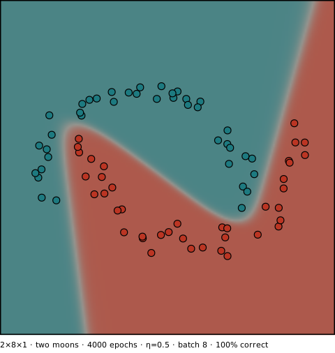
With JavaScript on, this becomes a sandbox: drop your own two classes of points, pick a hidden-layer shape, set the learning rate and batch size, and watch the boundary bend as it trains.

Things worth trying:

• XOR with 2×2×1. Two hidden units is the textbook minimum for XOR and it really is enough: every seed I tried had all forty points inside a few hundred epochs. The boundary arrives as two straight folds, which is exactly the two hidden units.
• The circle, then take a unit away. 2×4×1 fences it in at 100%. 2×2×1 tops out around 92%: two folds cannot close a region, so it settles for a wedge, and you can watch it try.
• The spiral with 2×4×1, that is the Challenge: break it button. Four sigmoid folds are not enough for an arm that wraps round nearly twice, and it plateaus at 60-70% correct however long you leave it; no learning rate rescues that. 2×8×1 gets to the low nineties and 2×8×8×1 past 95%, but both want a few thousand epochs, so turn epochs/frame up before you start.
• Turn the batch size up without touching η. The step size readout is $\eta B$, because of the summed-not-averaged update above. The average δ over the batch checkbox switches to the behaviour you probably expected; it is not what the repo does.

Export JSON writes out the weight vector in exactly the layout the Python class uses, each layer’s (nOut × nIn) block followed by its nOut biases, along with your points, so a network you like is a file you can keep, and Import takes it back.

Did it actually work

Two unit tests, and they test very different things.

UnitTests/BackPropTest1.py is a single step against a published worked example. It builds a 2×2×2 network from twelve fixed weights, forward-propagates [0.05, 0.1], backward-propagates towards [0.01, 0.99] at $\eta = 0.5$, and prints the network so you can compare every number by hand. Running the port in this post’s widget on those exact weights gives outputs 0.751365070 and 0.772928465, for an error of 0.298371109, matching the reference to nine decimal places.

There is one discrepancy, and it is instructive. After the update the reference gets 0.291028 and my network gets 0.280471. The reference walkthrough updates the eight weights and leaves the two biases where they started; equation 4.15 has no reason to treat a bias differently from any other weight, so my implementation updates all twelve. Freeze the two biases and it reproduces 0.291028 exactly.

UnitTests/BackPropTest2.py is the opposite kind of test: a 3-bit binary counter, so eight input patterns mapped to their successors, trained on a 3×5×5×3 network for 100,000 passes with $\eta = e^{-\text{loop}/50000 - 2}$. There is no reference to compare against, it just has to converge, on a problem with two hidden layers, which is the smallest thing that exercises the recursion rather than just the output-layer delta.

For the widget I added a third check the 2018 code does not have: a central-difference comparison of the analytic gradient against $\bigl(E(w+h) - E(w-h)\bigr)/2h$ for every weight in the vector, on 2×4×1, 2×4×2×1 and 2×8×8×1. It runs once on mount in development and logs the worst relative error, which comes out at about $10^{-7}$. That check has to run in double precision, incidentally: the training path uses Float32Array so the 128×128 heat map stays cheap, and in single precision the difference between $E(w+h)$ and $E(w-h)$ has no significant digits left in it, so the same check run in Float32 reports a relative error of 0.2 and looks like a broken gradient. If I had written any of this in 2018, the transpose in equation 4.14 would never have made it into the report.

The learning rate

One parameter, and the only one plain backprop has. The report’s Table 2 (p. 17) gives it as: η exponentially decays from 0.8 at epoch 1 to 0.005 at epoch 25 and higher. The runner implements that as a linear interpolation in log space, FFNNBackPropTestProben1.py lines 72 and 112:

for currentHiddenLayer, minMaxLearingRate in zip(datasetHiddenLayers, np.log(minMaxLearingRates)):
    ...
                learningRate=np.exp(np.interp(epoch, [0,25], minMaxLearingRate))

np.interp clamps outside its range, so the rate falls geometrically by a factor of 160 across the first twenty-five epochs and then simply sits at 0.005 for the rest of training. Coarse search first, then a long polish.

What this is for

Backpropagation as derived above is the baseline. It has one global learning rate, it is governed entirely by the magnitude of the gradient, and that magnitude is a number that gets small for two completely different reasons: because you are near a minimum, and because you are on the flat tail of a sigmoid four layers away from the error. The algorithm cannot tell those apart, which is what you are watching whenever a weight map in the sandbox above freezes into a solid block.

The rest of this assignment was ten more training algorithms, all of them attempts to fix that. The most interesting of them start by throwing the gradient’s magnitude away entirely, and that is the RPROP family, next.