Blog · Neural networks from scratch ·
The RPROP family: four ways to ignore the gradient's magnitude
RPROP keeps the sign of the gradient and throws the size away. Four variants, three lines of difference each, and visibly different trajectories.
- interactive
- neural-networks
- optimisation
- rprop
- numpy
The second half of the EAI732 assignment was to implement eleven training algorithms by hand and race them. Four of the eleven are the same algorithm with three lines changed, and they turned out to be the most interesting thing in the whole 349-page report: not because they won, though one of them did, but because they are built on a decision that sounds obviously wrong the first time you hear it.
RPROP throws away the magnitude of the gradient.
Gradient magnitude is a liar
Backpropagation’s update is . The size of the step is the size of the gradient times a global learning rate, and both halves of that are trouble. The learning rate is global, so a weight in a flat region and a weight on a cliff get the same treatment. And the gradient’s magnitude, in a deep or recurrent net, is the product of a long chain of partial derivatives: if those are individually less than one, the product decays as it is propagated backwards until the early layers receive nothing worth acting on. That is Hochreiter’s vanishing gradient problem, and it is the report’s stated reason for caring about RPROP at all.
RPROP’s answer is to use the gradient only for its direction, and to maintain the step size separately, per weight, from the history of that direction. If the sign of is the same as it was last iteration, then the minimum is still ahead of you, so take a bigger step next time. If it flipped, you just stepped over the minimum, so halve the step. Nothing about how steep the surface is enters into it.
The one rule
Every variant shares this. Let be the product of the current and previous gradients for one weight. Then
with . The weight then moves by in the
downhill direction. In NumPy that whole case analysis is two nested np.where calls, and
it is byte-for-byte identical in all four variants:
prevDw_times_Dw = self.dE_dw_t * self.dE_dw_t_m1

# implement prevDw_times_Dw>0 ->self.eta_plus
# prevDw_times_Dw<0 ->self.eta_minus
# else 1.0
deltaUpdate = np.where(prevDw_times_Dw > 0, self.eta_plus,
             np.where(prevDw_times_Dw < 0, self.eta_minus, 1.0))
self.delta = np.clip(self.delta * deltaUpdate, self.delta_min, self.delta_max)
Because is a multiplier, a weight that keeps agreeing with itself accelerates geometrically: with , thirty consecutive agreements multiply the step by 237. A weight that oscillates gets halved just as fast. This ratchet is the whole algorithm, and it is the one thing no textbook draws. That is why there is a strip under the contour plot below.
RPROP−: no bookkeeping at all
The simplest variant (report §5.1, Algorithm 3). Update the deltas, then step:
procedure RPROP-(w, Δ(t-1), ∂E/∂w(t), ∂E/∂w(t-1), η+, η-, Δmin, Δmax)
    h  ← ∂E/∂w(t) · ∂E/∂w(t-1)
    Δ(t) ← grow by η+ if h > 0, shrink by η- if h < 0, unchanged if h = 0
    w  ← w - sign(∂E/∂w(t)) · Δ(t)
end procedureRProp_minus_batch.updateWeights, after the delta update above:
self.neuralNetwork.weights -= np.sign(self.dE_dw_t) * self.delta

self.resetDE_Dw()
Two lines. On the iteration where the sign flips, a coordinate still takes a full step (a smaller one, in the new direction), which is exactly the behaviour the other three variants each try to improve on in a different way.
RPROP+: undo the last step
Report §5.2, Algorithm 4: when the gradient changes direction, revert the weight to where
it was before the last step, and zero the stored gradient so the next iteration sees
and leaves the delta alone. RProp_plus_batch.updateWeights:
self.delta_W = np.where(prevLessZero, self.delta_W, np.sign(self.dE_dw_t) * self.delta)

self.neuralNetwork.weights -= self.delta_W

self.dE_dw_t = np.where(prevLessZero, 0, self.dE_dw_t)
self.resetDE_Dw()iRPROP+: backtrack only if the error got worse
The improvement (§5.3, Algorithm 5) is small and sensible: reverting the weight is only worth the wasted iteration if the last step actually made things worse. So carry the total error from the previous batch and compare.
procedure iRPROP+(w, Δ(t-1), ∂E/∂w(t), ∂E/∂w(t-1), η±, Δmin, Δmax, E(t), E(t-1))
    h  ← ∂E/∂w(t) · ∂E/∂w(t-1)
    Δ(t) ← grow / shrink / hold, as above
    ∂E/∂w(t-1) ← 0 if h < 0, else ∂E/∂w(t)
    Δw(t) ← backtrack   if h ≠ 0 and E(t) > E(t-1)
            0           if h ≠ 0 and E(t) ≤ E(t-1)
            Δw(t-1)     if h = 0
    w ← w - Δw(t)
end procedure
The entire variant is one line of NumPy, iRProp_plus_batch.updateWeights:
self.delta_W = np.where(prevLessZero, self.delta_W if self.currentErr > self.prevErr else 0, np.sign(self.dE_dw_t) * self.delta)Note what kind of conditional that is. self.currentErr > self.prevErr is a plain Python
ternary evaluated once per call, on two scalars, not element-wise. So every flipped
weight in the network takes the same branch together: either they all repeat their last
step, or they all stand still. That is faithful to the algorithm as published (the error
is a property of the whole net, not of one weight), but it does mean the “improvement”
in iRPROP+ is gated on a single global number.
The extra bookkeeping this needs is the only place the four variants differ structurally.
iRProp_plus_batch overrides three methods of the batch base class purely to keep the
error in sync with the mini-batch accumulation: populateDE_Dw seeds currentErr with
the first pattern’s error, addToDE_Dw accumulates the rest, and resetDE_Dw rolls
currentErr into prevErr when the batch is flushed.
iRPROP−: just wait a turn
§5.4, Algorithm 6, and my favourite of the four for how little it costs. Don’t backtrack, don’t track the error; on a flip, set the gradient to zero before using it:
self.dE_dw_t = np.where(prevLessZero, 0, self.dE_dw_t)

self.neuralNetwork.weights -= np.sign(self.dE_dw_t) * self.delta
np.sign(0) is 0, so that weight does not move at all this iteration. Its delta has
still been halved, and its stored gradient is zero, so next iteration and the
delta holds. The weight sits out one turn with a halved step and then carries on. One
extra line over RPROP−, and on the cancer panels below it is indistinguishable from
iRPROP+. In fact, it is the first of the four to reach its floor.
Batching, and where the gradients come from
The batch classes never see a single pattern’s gradient. baseRPROP_batch
plays a small trick: updateDE_Dw is a field pointing at populateDE_Dw for the first
pattern of a mini-batch (which assigns into dE_dw_t) and is then rebound to addToDE_Dw
(which accumulates with +=) for the rest. resetDE_Dw swaps the two gradient buffers
rather than copying them and rebinds the field, so the next batch overwrites the older
buffer in place. The Proben1 runners call updateDE_Dw per pattern and updateWeights
once per mini-batch of at most 30 items.
The hyperparameters actually used
The four test runners, one per variant, all construct the optimiser as
RPROPTOTEST(NN) with no keyword arguments, so every run in the report used the same
constructor defaults, listed below:
| Parameter | Value |
|---|---|
| 1.2 | |
| 0.5 | |
| 0 | |
| 50 | |
| initial | np.random.uniform(0.005, 0.02) per weight |
| trials × datasets × architectures | 30 × 6 × (1–3) |
| mini-batch | ≤ 30 patterns |
| stopping | PQ, , epochs, first checked after epoch 5, cap 200 |
Watch the ratchet
This is the picture I wanted while writing the report and never drew. Pick a surface, tick the optimisers, drag the start point anywhere on the contour, and press Play. The strip below the plot is the part that matters: it is and for one optimiser on a log axis, so a run of agreeing gradients is a straight line climbing at a constant , and every triangle is an iteration where that coordinate’s gradient flipped sign and its step was multiplied by .
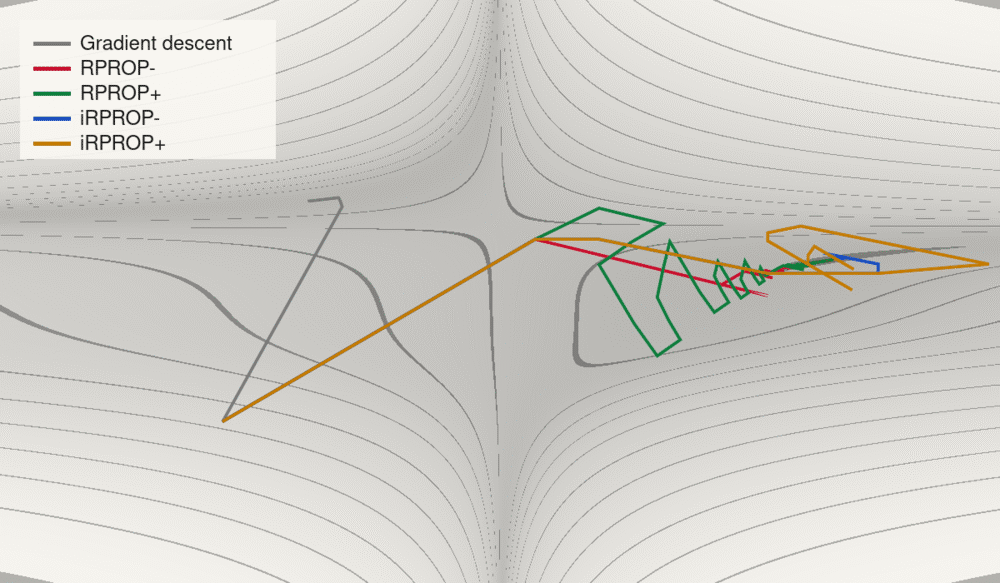
With JavaScript on this becomes an interactive race: four RPROP variants and plain gradient descent on a contour plot you can drag the start point around, with a step-size history strip underneath.
The optimisers in there are ports of the four batch classes, one coordinate pair standing in for the weight vector. I checked them against an independent line-by-line transcription of the NumPy: forty iterations of each variant on Rosenbrock from agree to 5 × 10⁻¹², which is the precision of the reference text file rather than a real disagreement.
Two things are worth doing in it. Turn down to 1.00 and the whole family stops being able to move: the step size can only ever shrink, so it never recovers the scale it threw away. And set the start point right out in a corner of Beale, where the gradient is enormous: gradient descent immediately explodes, and the RPROP variants do not notice, because to them a gradient of 10⁵ and a gradient of 10⁻⁵ are the same instruction.
What the benchmark said
Each of the eleven algorithms was run 30 times on each of the six Proben1 datasets, on one to three architectures each, with PQ early stopping. Below is the RPROP panel for the cancer dataset on a 9×4×2×2 network.
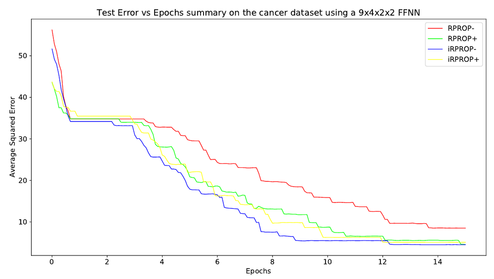
Report Figure 5, PDF p. 22 (printed p. 20). Average squared error percentage on the test set over 30 trials, cancer, 9×4×2×2. iRPROP− (blue) falls fastest; RPROP− (red) is slowest throughout and finishes around 8.5 where the other three settle near 5.
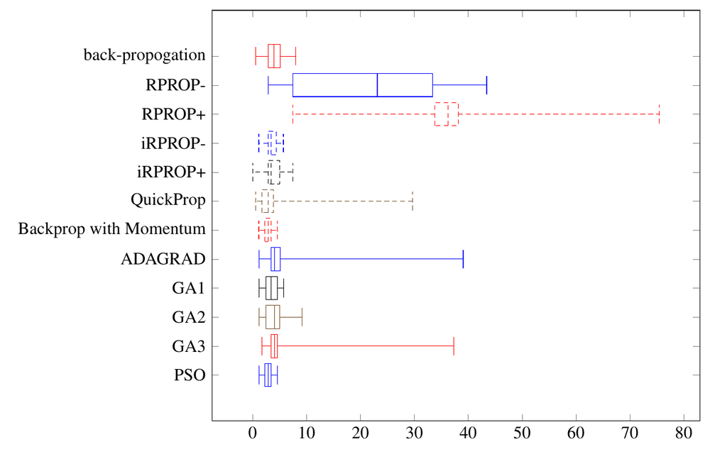
Report Figure 8, PDF p. 24 (printed p. 22). Best test error over 30 trials, same dataset
and architecture, for all eleven algorithms. RPROP− and RPROP+ are dramatically wider
than the two i variants, and RPROP+‘s upper whisker (out past 75 on the squared error
percentage scale) is the longest of any algorithm in the study.
The summary (§14, printed p. 58) puts it more plainly: “iRPROP+ showed excellent performance and was able to converge rapidly without any fine tuning.” That last clause is the real reason it won. Backpropagation needed a learning rate schedule decaying from 0.8 to 0.005 over 25 epochs, QuickProp needed and , momentum needed . The RPROP family ran on constructor defaults nobody ever touched.
What I take from it now
The interesting claim in RPROP is not “adaptive learning rates are good”: everything since has agreed on that. It is that the magnitude of the gradient is not just noisy but actively misleading, and that a method which never looks at it can beat one that does. Two decades on from Riedmiller and Braun, Adam still divides by a running , which is a smoothed way of arriving at roughly the same place: normalise the magnitude away, keep the direction.
The other lesson is the one in the callout above. A four-line variant with a missing minus sign went into every plot of a 349-page report and I did not notice, because it still trained, just badly, in a way that reads as variance. Writing the same four updates out again for this post, with a picture of the step sizes underneath it, found it in an afternoon. There is a “unit test” for all four: each one trains a 3×100×3 net to count in binary and prints the error every step. Not one of them contains an assertion. A test that a human has to read is a test that catches the bugs which look wrong, and this one looked fine.
Next in this series: the same racer with QuickProp, ADAGRAD and momentum added, which are three quite different bets about what the error surface looks like. After that, the same contour gets a population of 64 creatures on it, for the genetic algorithms and PSO.