Blog · Research infrastructure ·
Every number you can call 'accuracy' for a semantic map
Point accuracy, mean class accuracy, IoU, mIoU and FIoU disagree about the same prediction. Ported from a 2019 benchmark harness's metrics.py, with a widget that lets you win on one and lose on another.
- interactive
- python
- semantic-segmentation
- evaluation-metrics
- computer-vision
- research-infrastructure
Look at one row of the table my evaluation platform produced for SemanticFusion on ScanNet: 54.5% accuracy on Wall, 43.0% on Floor, 0.05% on TV. That is not SemanticFusion being bad at televisions specifically. It is what “accuracy” does to a class that is a few dozen pixels in a room where the walls and floor are most of the points. A method that has never seen a television can still score 99.95% accuracy on “is this a television” by never predicting one, because “accuracy” only asks whether the label at each point was right, and almost no points are TVs.
This is the unglamorous half of the masters project I keep coming back to in this series: not the algorithms, but the harness that scored them the same way, every time, so the numbers above were comparable at all. The metrics module is a compact 124 lines and five different definitions of “how good is this prediction” that all sound like the same question and are not. This post ports every one of them to TypeScript, quotes the real numbers they produced, and (because two of the four algorithms under test were never even trained on three of the thirteen classes) spends a section on the part nobody writes about: before you can average anything, two datasets have to agree on what a “class” is.
Point accuracy lies by omission
# segtester/metrics/seg.py:4-5
def point_accuracy(est_labels, gt_labels):
    return np.count_nonzero(est_labels == gt_labels), gt_labels.size
Two numbers, a numerator and a denominator, and that is the entire function: every point where the prediction matches the label, over every point. It is the number everyone quotes first because it is the easiest to explain, and it is also the number that rewards predicting the majority class and ignoring everything else, because most points in an indoor scan are wall or floor. The widget at the end of this post lets you prove that to yourself in one click.
Mean class accuracy: average over classes, not points
# segtester/metrics/seg.py:8-19
def class_accuracy(est_labels, gt_labels, all_labels=None):
    if all_labels is None:
        all_labels = np.unique([est_labels, gt_labels])
    all_to_gt = all_labels[:, None] == gt_labels[None]
    all_to_est = all_labels[:, None] == est_labels[None]
    return np.count_nonzero(np.logical_and(all_to_gt, all_to_est), axis=1), \
           np.count_nonzero(all_to_gt, axis=1), \
           all_labels


def mean_class_accuracy(class_accuracies, exclude_background=True):
    return np.nanmean(class_accuracies[int(exclude_background):])
class_accuracy builds two boolean matrices (“is this ground-truth point class c”,
“is this predicted point class c”) for every class in all_labels at once, and counts
true positives and ground-truth totals per class in two broadcasted comparisons rather
than one loop per class. mean_class_accuracy then averages per-class accuracy, not
per-point: a class with 40 points and 90% accuracy counts exactly as much as one with
40,000 points and 90% accuracy. exclude_background=True slices off index 0 before
averaging, which is why int(exclude_background) (True is 1 in Python) is doing
double duty as a boolean flag and a slice offset in the same expression. This is the
metric that punishes “predict wall everywhere” properly: every class the prediction never
touches scores 0%, and 0% counts the same as any other class’s 0%, majority or not.
IoU, mIoU, and the NaN that has to survive
# segtester/metrics/seg.py:22-33
def iou(est_labels, gt_labels, all_labels=None):
    if all_labels is None:
        all_labels = np.unique([est_labels, gt_labels])
    gt_eq_label = all_labels[:, None] == gt_labels[None]
    est_eq_label = all_labels[:, None] == est_labels[None]
    intersection = np.count_nonzero(np.logical_and(gt_eq_label, est_eq_label), axis=1)
    union = np.count_nonzero(np.logical_or(gt_eq_label, est_eq_label), axis=1)
    return intersection, union


def miou(iou):
    return np.nanmean(iou)
Intersection over union per class, then averaged. The part worth pausing on is what
happens when a class is absent from both the prediction and this particular
comparison: union is 0, intersection / union is 0 / 0, and numpy gives you nan, not
an error, not a silent zero. np.nanmean in miou then skips that class rather than
counting it as a zero. That distinction is the entire reason the - marks in the tables
below exist, and I nearly missed it the first time I read this file, because a stray
np.mean instead of np.nanmean would silently turn “this class doesn’t apply here”
into “this class scored zero here”, a very different number.
FIoU sits between the other two on purpose
# segtester/metrics/seg.py:36-43
def fiou(est_labels, gt_labels, all_labels=None):
    if all_labels is None:
        all_labels = np.unique([est_labels, gt_labels])
    gt_eq_label = all_labels[:, None] == gt_labels[None]
    est_eq_label = all_labels[:, None] == est_labels[None]
    t_i = np.count_nonzero(gt_eq_label, axis=1)
    return np.nansum(t_i * np.count_nonzero(np.logical_and(gt_eq_label, est_eq_label), axis=1) /
                     np.count_nonzero(np.logical_or(gt_eq_label, est_eq_label), axis=1)) / t_i.sum()
Frequency-weighted IoU: the same per-class IoU as above, but weighted by t_i, how many
ground-truth points that class actually has, before averaging. A class with one point
that scores IoU 1.0 barely moves FIoU; the same class would move mIoU exactly as much as
Wall does. Every row of the results table below shows FIoU landing between raw accuracy
and mIoU, which makes sense once you see it as “accuracy, but a class only gets credit
for the fraction of its points it also didn’t steal from someone else,” rather than
“accuracy” straight.
Two datasets never agree on what a “class” is
Every metric above takes all_labels (the fixed set of classes to score, passed in
explicitly rather than computed from whatever happens to be present in one scene. That
matters because ScanNet’s raw labels, NYUv2’s raw labels, and “the 13 classes I actually
want a comparable number for” are three different vocabularies, and someone has to
collapse them onto one before any of the metrics above mean anything across datasets.
That collapse is a CSV and about a dozen lines of numpy:
# segtester/labelmaps/csv_label_map.py:9-29
def get_label_text(self, id_col_name, text_col_name, default_value='object', default_key=0):
    max_from_label = 0
    label_map = {}
    default_set = False
    with open(self.csv_path, mode='r') as csv_file:
        reader = csv.DictReader(csv_file)
        for row in reader:
            if str(default_key) == row[id_col_name]:
                default_set = True
            key = int(row[id_col_name]) if row[id_col_name] != '' else default_key
            val = row[text_col_name]
            max_from_label = max(max_from_label, key)
            if key not in label_map:  # take the first one matching
                label_map[key] = val
    if not default_set:
        label_map[default_key] = default_value
    labels = np.array(list(label_map.values()))
    np_label_map = np.repeat(np.array(default_value, dtype=labels.dtype), max_from_label+1)
    np_label_map[list(label_map.keys())] = labels
    return np_label_map
get_label_text reads a CSV where one column is a raw dataset id (ScanNet’s nyu40id,
say) and another is the target taxonomy’s id (eigen13id), and builds a plain numpy
array where array[raw_id] gives you the target id, so remapping an entire label image
is one fancy-index operation, np_label_map[image], not a per-pixel loop. A sibling
function, get_label_map, which the wrapper Segmentation3DAssessment.__init__ actually
calls, does the same thing for numeric ids on both sides. Neither the CSV nor the raw dataset ids are committed to the repository (this is
personal-filesystem plumbing I never checked in) but the effect is checkable, because
the harness passes a fixed, explicit all_class_ids into every metric call rather than
deriving it per scene:
# segtester/assessments/segmentation3d.py:55, 141-157
all_class_ids = np.array(self.label_map.get_unique_values(self.conf.label_map_dest_col), dtype=np.int)
...
@staticmethod
def get_results(est_labels, gt_labels, class_ids=None):
    pt_acc_num, pt_acc_den = smet.point_accuracy(est_labels, gt_labels)
    inst_acc_num, inst_acc_den, _ = smet.class_accuracy(est_labels, gt_labels, class_ids)
    mca = smet.mean_class_accuracy(inst_acc_num / inst_acc_den)
    i, u = smet.iou(est_labels, gt_labels, class_ids)
    with np.errstate(divide='ignore', invalid='ignore'):
        iou = i/u
    miou = smet.miou(iou)
    fiou = smet.fiou(est_labels, gt_labels, class_ids)
    ...
class_ids here is always the full 14-id set from the label map (13 named classes plus
background), never np.unique([est, gt]) for the scene at hand. That is a deliberate
choice with a real consequence: a scene that happens to contain no chairs still gets a
“Chair” slot in its per-class arrays (nan, not absent) so averaging across scenes
later doesn’t silently redefine what “mIoU” means from one scene to the next depending on
what walked into frame. Derive all_labels from the data instead, and a scene with no
chairs quietly stops being penalised for missing chairs at all, because there was never a
chair-shaped slot to score.
What the - in the table actually means
| Class | Acc. 3DMV | Acc. ME 2cm | Acc. ME 5cm | Acc. SF | IoU 3DMV | IoU ME 2cm | IoU ME 5cm | IoU SF |
|---|---|---|---|---|---|---|---|---|
| Bed | 58.121 | 95.188 | 30.597 | 25.744 | 0.089 | 0.310 | 0.102 | 0.039 |
| Books | – | – | – | 47.457 | – | – | – | 0.012 |
| Ceiling | – | – | – | 7.570 | – | – | – | 0.023 |
| Chair | 80.997 | 89.511 | 51.555 | 14.146 | 0.353 | 0.638 | 0.236 | 0.077 |
| Floor | 94.192 | 97.958 | 95.764 | 42.992 | 0.785 | 0.859 | 0.737 | 0.345 |
| Furniture | 59.140 | 86.057 | 32.747 | 28.317 | 0.261 | 0.591 | 0.151 | 0.132 |
| Objects | 4.510 | 9.855 | 0.138 | 22.690 | 0.046 | 0.094 | 0.002 | 0.109 |
| Picture | 15.990 | 72.211 | 1.259 | 14.115 | 0.054 | 0.358 | 0.011 | 0.027 |
| Sofa | 26.607 | 97.112 | 11.989 | 17.498 | 0.062 | 0.345 | 0.036 | 0.029 |
| TV | – | – | – | 0.048 | – | – | – | 0.000 |
| Table | 72.075 | 95.242 | 35.995 | 12.763 | 0.350 | 0.591 | 0.144 | 0.061 |
| Wall | 66.771 | 98.406 | 93.802 | 54.481 | 0.463 | 0.676 | 0.503 | 0.299 |
| Window | 67.983 | 90.788 | 47.803 | 16.464 | 0.155 | 0.552 | 0.209 | 0.059 |
Objects is the row I keep pointing people at: 3DMV 4.5%, ME 5cm 0.14%, ME 2cm 9.9%, every voxel-grid method is close to blind to it, against SemanticFusion’s 22.7%. A coarse voxel loses anything smaller than a voxel; an image-space method that fuses per-frame CNN predictions doesn’t have that floor.
The full picture, and where FIoU sits
| Algorithm | Class. Acc. [%] | Class. FIoU | Class. MIoU | Inst. Acc. [%] | Inst. FIoU | Inst. MIoU | Sem. Acc. [%] | Sem. FIoU | Sem. MIoU |
|---|---|---|---|---|---|---|---|---|---|
| 3DMV | 57.316 | 0.459 | 0.373 | 48.034 | 0.392 | 0.044 | 40.815 | 0.340 | 0.032 |
| ME (2cm) | 73.592 | 0.695 | 0.681 | 54.407 | 0.448 | 0.214 | 50.831 | 0.419 | 0.175 |
| ME (5cm) | 54.922 | 0.442 | 0.288 | 38.349 | 0.276 | 0.085 | 31.551 | 0.219 | 0.044 |
| SemanticFusion | 34.325 | 0.207 | 0.161 | 26.036 | 0.208 | 0.010 | 20.942 | 0.160 | 0.007 |
Every row, FIoU sits between accuracy and MIoU, exactly as the weighted-average argument above predicts. ME (2cm) also makes the earlier “voxel size mattered more than architecture” point on its own: the same network at 5cm loses 18.7 points of classification accuracy, a bigger drop than the 16.3-point gap between two entirely different architectures (3DMV vs ME 2cm).
The same three metrics, reprojected into 2D: a discrepancy I found
The NYUv2 numbers come from a second pipeline, the 2D reprojection driver, that reprojects
SemanticFusion’s 3D map back through a camera and scores it against the 2D ground truth
with the identical get_results function:
| SemanticFusion | Accuracy [%] | FIoU | MIoU |
|---|---|---|---|
| Classification | 37.166 | 0.248 | 0.145 |
| Instance Segmentation | 1.433 | 0.010 | 0.003 |
| Semantic Segmentation | 21.471 | 0.182 | 0.045 |
Reading the two assessment drivers side by side turned up something the report (there
isn’t one, only the code) never says out loud. The 3D assessment driver masks out every
point whose ground truth is unlabelled before it ever calls get_results:
# segtester/assessments/segmentation3d.py:99-101
non_zero_mask = mapped_gt_seg.classes!=0
seg_3d_est = seg_3d_est.get_masked_seg(non_zero_mask)
mapped_gt_seg = mapped_gt_seg.get_masked_seg(non_zero_mask)
The 2D reprojection driver has no equivalent step anywhere before its own get_results
calls. The 3D numbers above are
computed only over points where the ground truth actually says something; the 2D NYUv2
numbers include every pixel NYUv2 left unlabelled, scored as class 0 against whatever
SemanticFusion happened to predict there. That is not a bug I can point to a single wrong
line for, both pipelines call the same, correct get_results, but it is a genuine,
checkable difference in what “ground truth” means between the two assessments in the same
codebase, and it means the 3D and 2D numbers in this post are not measuring quite the same
thing even though they share every metric function.
Decoding a label image with no key
The renders in this post and the widget below use a fixed colour scheme with no legend
file anywhere: the 3D point-cloud renderer (get_labelled_pcd, used for the ScanNet
point clouds) and the 2D image renderer (vis_labels, used for the NYUv2 pairs below)
both do the same three lines:
# segtester/types/seg2d.py:39-48 (seg3d.py's get_labelled_pcd is identical in spirit)
cmap = plt.get_cmap("hsv")
if labels_to_vis is None:
    labels_to_vis = self.classes
max_class = labels_to_vis.max()
vis_cmap = cmap((np.arange(max_class+1)-1)/max_class)
vis_cmap[0] = (0.3, 0.3, 0.3, 1)
Class 0 always renders as a fixed grey; class i ≥ 1 renders as
hsv_cmap((i - 1) / max_class). The part that makes this genuinely undecodable without
reading the source: max_class is labels_to_vis.max(), the highest class id present in
that one image, neither function is ever called with a fixed value in this codebase.
Two renders of the same 13-class taxonomy can legitimately use two different palettes,
because they happened to top out at different ids. I checked this against every one of the
34 NYUv2 ground-truth/estimate frame pairs: max_class is 7, 12 or 13 depending on which
classes happen to be in frame.
I also learned, the annoying way, that matplotlib’s "hsv" colormap is not a plain
hue = x wheel: it disagrees with colorsys.hsv_to_rgb(x, 1, 1) by up to 24 of 255 in a
channel, and it quantises to a fixed 256-entry internal table rather than evaluating
continuously. Decoding these images means reproducing that exact table, not a
mathematically-tidier approximation of it.
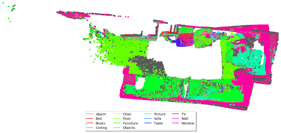
This render, the one in the source repository with its own legend baked in, is what let
me confirm the class order used throughout this post: alphabetical, object (background)
first. Credit: ScanNet (Dai et al.) scene geometry and labels; render is the harness’s
own code.
Paint a prediction
Two 32×24 grids. The left one is seeded from a real NYUv2 frame, decoded client-side from the actual PNG, the same technique as the section above, not a synthetic bitmap. The right one starts blank; paint it with the 14-class brush and every metric on this page recomputes on every stroke. Predict the majority class everywhere and watch point accuracy jump while mIoU collapses to whatever one class’s IoU happens to be, because every other class the ground truth actually contains just scored zero. Get the small objects right, miss the rest does the opposite on purpose: it copies the ground truth everywhere except the frame’s two most common classes, which it deliberately gets wrong. Point accuracy drops hard, because those two classes are most of the image, but mean class accuracy and mIoU read far better than the first preset, because every minority class scores a perfect 1.0. The same prediction, two verdicts.
The second tab switches from a painting exercise to the real thing: the actual ground-truth/estimate pixel pair for the selected frame, decoded and scored in your browser exactly the way the table two sections up was produced. Not read from a pre-computed results table: computed from the pixels. A confusion matrix (hover or focus a cell for its count), an undo stack, and a copy-the-metrics button are there because a widget that only shows you numbers once is a demo; one you can poke at your own frame is a small tool.
With JavaScript enabled, this becomes a 32×24 painting grid with a live metrics readout, two one-click presets, a confusion matrix, and a second tab that decodes and scores one of 34 real NYUv2 ground-truth/estimate pairs in your browser.
Static fallback: the ScanNet legend render above.
What I’d tell past me
Report one number and you’ve made a choice, whether or not you say so. Point accuracy tells you what fraction of a scan you’d colour correctly if you were painting by hand, useful, and it will make a wall-and-floor detector look excellent. Mean class accuracy tells you how the method does on an average class, not an average point, which is the number that actually punishes ignoring TVs. IoU per class, and its two averages, tell you whether a class’s predicted extent overlaps its true extent, which accuracy alone can’t: a method that predicts “wall” for exactly the wall pixels and a method that predicts “wall” for the wall pixels plus half the room can have identical wall accuracy and very different wall IoU. None of the five is wrong. They’re different questions, and “accuracy” is not specific enough to say which one you asked, which is exactly why every results table in this post reports all three, side by side, instead of picking a winner.