Blog · Segmentation ·
Mean shift, or how to segment an image without knowing how many regions there are
Pixels are a point cloud in Luv space; every region is a bump in its density. Comaniciu & Meer's three practical hacks (random search windows, a connected-component sanity check, and a radius-expansion pass) turn that idea into an algorithm.
- interactive
- segmentation
- mean-shift
- clustering
- connected-components
- wasm
k-means makes you commit to a number up front. Tell it “5 clusters” and it will hand you exactly 5, whether or not the picture actually contains five things. Mean shift refuses that question. It treats every pixel as a point in colour space, notices that a region of the photograph is really just a bump in the density of that point cloud, and finds the bumps by climbing them, however many there turn out to be.
This is the report’s Section 7.1, and it belongs to Comaniciu and Meer, whose two papers
turn a one-paragraph idea into something you can actually run on a photograph: random
search windows instead of a walk per pixel, a sanity check that a colour cluster has to
pass in the image, not just in colour space, and a radius-expansion pass to sweep up
what is left over. That middle step (a cluster is only accepted if it forms a connected
blob of at least N_min pixels in the image) is the one most write-ups skip, and it is
the one this post is actually about.
A point cloud with bumps in it
Convert an image from BGR to Luv and every pixel becomes a point in a 3-D colour space where Euclidean distance is roughly perceptual distance: two points close together in Luv really do look like similar colours, which is not true of raw RGB. A region of the photograph (the sky, a roof, a face) is a lot of pixels with nearly the same colour, so it shows up as a dense cluster of points. Find the dense clusters, and you have found the regions.
Algorithm 1 of the report is the whole idea, seven lines long:
procedure MEANSHIFT(Initial Point (p), Feature Vectors (F), Window radius (r), Convergence Threshold (α))
    repeat
        μ ← p
        Indices ← i where ‖Fᵢ − p‖₂ ≤ r
        p ← Mean(F[Indices])
    until ‖μ − p‖₂ < α
    return p
end procedure
Drop a window of radius at a point, take the mean of every feature vector inside it, move there, repeat. Each move is a step toward wherever the local density is highest: literally the mean shift the algorithm is named for, and the walk stops once it settles, at . Every point that walks to (nearly) the same place belongs to the same region.
The report names two problems with this in its raw form. First, run it as written and you have to start a separate walk from every pixel: for a modest photograph that is tens of thousands of walks. Second, a point that starts almost exactly between two modes can stall in the gap, pulled equally by both and settling nowhere useful. The fix for the second problem the report offers is a Gaussian-weighted mean instead of a flat one, so points closer to the current estimate count for more. Comaniciu and Meer’s five steps solve the first:
- Map the image into feature space (RGB to Luv transformation).
- Define random search windows across the feature space.
- Find regions of high density by applying the mean-shift algorithm.
- Validate the extracted centres in both the image domain and feature space.
- Allocate the remaining pixels.
Step 3 runs the walk from only the densest of random starting windows, not from every pixel: one walk finds one region, and the pixels it claims are removed from consideration before the next window is drawn. That is the whole trick that makes this tractable on a real photograph.
The five steps, as code
The Python implementation is 265 lines, and its mean_shift_alg function covers steps
1 to 5 in order. Step 1, the colour-space mapping, plus a second, 3×3-box-filtered copy of
the same image that step 2’s candidates are drawn from:
def mean_shift_alg(img, param_mode=0):
    mean_img = cv2.boxFilter(img, cv2.CV_8U, (3, 3))
    feature_space_img = cv2.cvtColor(img, cv2.COLOR_BGR2Luv)

    image_co_ordinates = get_image_indicies(img)
    flat_feature_space_img = feature_space_img.reshape((-1, feature_space_img.shape[-1]))
    flat_feature_space_mean_img = cv2.cvtColor(mean_img, cv2.COLOR_RGB2Luv).reshape((-1, feature_space_img.shape[-1]))
I double-checked that cv2.COLOR_RGB2Luv line more than once while porting this, and it
really is the wrong conversion constant, not a typo I am misreading. mean_img was
box-filtered from img, which cv2.imread hands back as BGR, exactly like
feature_space_img two lines above it. Converting the same byte-order array with
RGB2Luv instead of BGR2Luv silently swaps the red and blue channels of every candidate
window’s starting colour. It does not corrupt the final result: get_close_point
immediately converges using the correctly converted flat_feature_space_img, so a
mis-hued candidate is only ever a slightly-wrong place to start climbing from, not a wrong
answer. Still, it is a genuine slip, and a fun one to turn up while revisiting old work. I did not
reproduce it in the Rust port (more on that below).
Step 2 and step 3: draw random candidates from the box-filtered image, count how many real pixels fall within of each, and mean-shift the best one:
sigma = np.std(feature_space_img.flatten())
params = Parameters(sigma, param_mode)
M = 200
clusters = []

while True:
    if len(flat_feature_space_mean_img) <= 0:
        break
    feature_space_candidate_pixels = flat_feature_space_mean_img[np.random.randint(0, len(flat_feature_space_mean_img), M)]

    dist_from_center = np.sum(np.square(flat_feature_space_img[:, None]-feature_space_candidate_pixels), axis=2)

    num_in_each_window = np.sum(dist_from_center <= params.r_sq, axis=0)
    ind_most_in_window = np.argmax(num_in_each_window)

    if num_in_each_window[ind_most_in_window] < params.N_min:
        break

    mode, ind_in_radius = get_close_point(feature_space_candidate_pixels[ind_most_in_window],
                                          flat_feature_space_img, params.r_sq, 0.01, -1)
np.std(feature_space_img.flatten()) is worth pausing on: it is one standard
deviation over every L, u and v value pooled together into a single 1-D array, not a
per-channel . Whatever the report means by "" in , it is
this pooled number, and it is what makes the radius comparable across photographs with
very different colour ranges.
get_close_point is Algorithm 1 with the Gaussian weighting the report’s prose promised,
plus the guard that keeps it from dividing by zero:
def fast_isotropic_multivariate_gauss(neg_half_sigma, dists_squared_from_mean):
    hold_out = np.exp(neg_half_sigma*dists_squared_from_mean)
    if np.allclose(hold_out, 0):
        return np.ones(hold_out.shape)
    return hold_out

def get_close_point(test_point, point_list, test_radius_squared, stop_criteria, neg_half_sigma):
    delta = stop_criteria + 1
    while not delta < stop_criteria:
        square_dists = np.sum(np.square(point_list - test_point), axis=1)
        ind_in_radius = np.where(square_dists <= test_radius_squared)
        if len(ind_in_radius[0]) == 0:
            return test_point, ind_in_radius
        points_in_radius = point_list[ind_in_radius]
        weights = fast_isotropic_multivariate_gauss(neg_half_sigma, square_dists[ind_in_radius])
        new_test_point = np.average(points_in_radius, axis=0, weights=weights)
        delta = np.sum(np.square(new_test_point-test_point))
        test_point = new_test_point
    return test_point, ind_in_radius
get_close_point is called with stop_criteria=0.01 and neg_half_sigma=-1. delta is
a squared distance, so 0.01 is for the report’s stated :
consistent, once you notice the squaring.
The step that gets skipped: validating in the image domain
Step 4 is where this post earns its title. A mean-shift walk only ever looks at colour:
nothing in get_close_point knows or cares where in the image a point came from. So
before a discovered mode is accepted as a real region, mean_shift_alg checks it against
a second, completely different question: do these pixels actually sit next to each other
in the photograph?
class Cluster:
    def get_max_connected_components(self, imgshape):
        img_map = np.zeros(imgshape, dtype=np.int)
        img_map[self.image_coords['y_coord'], self.image_coords['x_coord']] = 1
        labeled, ncomponents = label(img_map, np.ones((3, 3), dtype=np.int))
        if ncomponents < 1:
            return 0
        return max([(labeled == i).sum() for i in range(1, ncomponents+1)])
This method paints the cluster’s pixels onto a blank image, runs scipy.ndimage.label
with an all-ones 3×3 structuring element (8-connectivity: a diagonal touch joins two
blobs), and returns the size of the largest single connected component, not the size of
the cluster. Back in mean_shift_alg:
accepted_clusters = []
for cluster in clusters:
    if cluster.get_max_connected_components(img.shape[:-1]) > params.N_min:
        accepted_clusters.append(cluster)
clusters = accepted_clusters
Colour similarity is necessary but not sufficient. A handful of red pixels scattered
across a photograph of a sunset (clouds here, a reflection there, a strip of brick two
rooms away) can easily beat N_min on colour count alone. Comaniciu and Meer’s insight
is that a region has to also be a region: a single connected blob, in the image, of
respectable size. Fail that and the whole colour cluster is thrown away, however tight it
was in Luv.
Peeling, expansion, and the orphans
Once a cluster is found (accepted or not), its pixels are removed from the pool before
the next candidate window is drawn, so the same dense region cannot be rediscovered twice.
get_coords_in_surrounding_radius removes not just the pixels the walk claimed but their
8-neighbours too, so accepted regions do not leave a jagged one-pixel-wide moat of
unclaimed pixels along every boundary:
new_ind_in_radius = get_coords_in_surrounding_radius(image_co_ordinates, ind_in_radius)
clusters.append(Cluster(mode, image_co_ordinates[ind_in_radius], flat_feature_space_img[ind_in_radius]))
image_co_ordinates = np.delete(image_co_ordinates, new_ind_in_radius[0], axis=0)
flat_feature_space_img = np.delete(flat_feature_space_img, new_ind_in_radius[0], axis=0)
flat_feature_space_mean_img = np.delete(flat_feature_space_mean_img, new_ind_in_radius[0], axis=0)
That loop runs until the best of the candidate windows holds fewer than N_min
points: nothing dense enough is left to find. Then the report picks up the story:
The process is repeated until the amount of pixels in the final search window is less than . Once it is done, each region is inspected to see if it contains connected regions in the image domain which are larger than . If this is not the case, the label is discarded. Now that the labels and the associated feature space centres are known, all pixels are unassigned. Pixels which now lie in the initial search window are assigned to the respective labels. The search window radius is then multiplied by in order to increase the window size. Points which now lie within the windows are also assigned to the respective label. The remaining pixels are assigned to the label which has the closest feature space representation to it.
The important sentence there is “all pixels are unassigned”. Once validation has decided which modes survive, the code throws every pixel’s peeling-phase membership away and starts over from the complete, untouched image:
flat_feature_space_img = flat_feature_space_img_2
image_co_ordinates = image_co_ordinates_2(flat_feature_space_img_2 was copied at the very top of the function, before the peeling
loop even ran.) So a discarded cluster is not a hole in the final picture: its pixels
simply go back into the general pool and get claimed by whichever accepted mode ends up
nearest, exactly like every other unclaimed pixel. What validation actually controls is
not “which pixels get coloured” but “which colours are allowed to exist as a region at
all”: every pixel in the photograph is assigned in the end, but only to a mode that
proved, at least once, that it was more than a scattering of similarly-coloured dots.
The assignment itself is two passes: first, every accepted mode’s capture radius grows by (which, since capture volume in 3-D scales with , exactly doubles the volume each mode can claim without changing its shape), and claims whatever is left within it; then everything still unclaimed goes to whichever mode is nearest in feature space.
The dial: four presets, one algorithm
Parameters.__init__ is a small lookup table that turns one number (which of four modes
to run in) into three: the search radius as a multiple of , the minimum accepted
size N_min, and N_con.
class Parameters:
    def __init__(self, sigma, parameter_type=0):
        if parameter_type == -1:
            self.r = 0.8*sigma
            self.N_min = 300
            self.N_con = 50
        elif parameter_type == 0:
            self.r = 0.4*sigma
            self.N_min = 400
            self.N_con = 50
        elif parameter_type == 1:
            self.r = 0.3*sigma
            self.N_min = 100
            self.N_con = 10
        else:
            self.r = 0.2*sigma
            self.N_min = 50
            self.N_con = 0
        self.r_sq = self.r*self.r
        expanded_r = self.r*(2.0**(1/3.0))
self.expanded_r_sq = expanded_r*expanded_r| preset | |||
|---|---|---|---|
| under-segmentation, more | 300 | 50 | |
| under-segmentation (report default) | 400 | 50 | |
| over-segmentation | 100 | 10 | |
| quantisation | 50 | 0 |
A bigger radius sweeps up more of the point cloud per walk, so fewer, larger modes survive:
under-segmentation. A smaller radius is pickier, so more, smaller modes survive:
over-segmentation, sliding toward quantisation as shrinks further. The script that
produces the report’s figures calls mean_shift_alg(img) with no param_mode argument,
so every figure in the report used the 0.4\sigma default.
Watch a walk climb
The widget below has two linked panes. Left is the photograph: click a pixel and its Luv colour seeds a mean-shift walk. Right is the image’s pixels binned into a density heatmap over the u–v plane, with lightness mapped onto a colour ramp: click there instead and the walk starts from the nearest bin. Either way, the walk always animates on the right: a polyline tracing every step, the current search window drawn as a circle, climbing toward a mode exactly like Algorithm 1 says.
Sliders set (as a multiple of ), N_min and N_con directly, or pick one of
the four presets above. Run full segmentation drives the whole pipeline (the peeling
loop, the image-domain validation, the expansion, the orphan assignment) and
shows a live accepted-versus-discarded count as it runs, flashing each cluster green if its
image footprint passed and hatched grey if it did not. Uncheck “validate in the image
domain” and run it again to see the difference validation actually makes.
With JavaScript on, this becomes an interactive explorer: click either pane to watch a mean-shift walk climb to a mode, adjust the radius, N_min and N_con sliders or pick a report preset, and run the full segmentation with a live accepted/discarded cluster count. You can drop in your own photograph and download the result.
Porting it to Rust: a rewrite, not a port, in one place
Most of mean_shift_alg translates line for line. One part does not: the peeling loop’s
repeated np.delete(image_co_ordinates, ind, axis=0) allocates a brand new array on every
single accepted cluster: an O(n) copy, tens of times, for an operation that is
conceptually “remove a few thousand indices from a set of tens of thousands”.
The Rust port’s ActivePool replaces that with swap-remove compaction: a flat index
array (list) plus an O(1) pos[] lookup from a flat pixel index to its current position
in list. Removing an element swaps it with the last live element and shrinks the array by
one: no shifting, no reallocation, no O(n) scan:
struct ActivePool {
    list: Vec<u32>,
    pos: Vec<u32>,
}

impl ActivePool {
    fn remove(&mut self, flat: u32) {
        let i = flat as usize;
        let p = self.pos[i];
        if p == u32::MAX { return; }
        let last = self.list.len() as u32 - 1;
        let last_flat = self.list[last as usize];
        self.list.swap(p as usize, last as usize);
        self.pos[last_flat as usize] = p;
        self.list.pop();
        self.pos[i] = u32::MAX;
    }
}
A test proves the two approaches agree: remove 300 of 500 indices in a random order
through ActivePool, and the surviving set (order ignored) is identical to a naive
filter over a removed[] boolean array.
The rest is a faithful, if occasionally corrective, port:
- No spatial channel. Unlike EM (post 42), the report never appends to mean shift’s feature vector. It is Luv, 3-D, throughout.
- The box-filtered candidate image is colour-correct. As covered above, the Python
converts
mean_imgwith the wrong constant (COLOR_RGB2Luvon a still-BGR array). The Rust box-filters the sRGB directly and converts with the samergb_to_luv8everything else uses: the same 3×3-averaging behaviour the report’s prose describes, minus the channel swap. - Connected components are 4-connected, not 8-connected. The union-find module
(shared with, and written for this post by, post 42) is 4-connected; the Python’s
scipy.ndimage.label(img_map, np.ones((3, 3)))is 8-connected, so a diagonal-only bridge between two blobs is occasionally seen as two components here where the original saw one. That can only make this port’s validation stricter, never looser: nothing this port accepts would have been rejected by the original. - Mode seeking is capped at 200 iterations.
get_close_point’swhile not delta < stop_criteriahas no bound; a WASM instance withpanic = "abort"cannot risk a pathological oscillation hanging the tab, so this port stops and returns the current estimate past 200 steps: a safety margin never observed to bind in testing (every case converges in under 40).
cargo test -p segment-wasm adds ten cases in the mean-shift module: a mode-seeking walk
on a synthetic two-blob point cloud converges to the right mode from either starting side;
the image-domain validation accepts a compact 4×4 block and rejects a colour cluster
sprinkled one pixel per 2×2 block (a checkerboard-like scatter that is, under
4-connectivity, all size-1 components); the swap-remove pool matches a naive filter after
300 random removals from 500; the expansion doubles capture volume to three
decimal places; the Gaussian-weight guard falls back to a flat mean when both test points
underflow; the four presets match the report’s table exactly; N_con pruning keeps a
16-pixel block and drops three 1-pixel satellites; skipping image-domain validation never
accepts fewer clusters than validating does; and a full end-to-end run on a two-colour
synthetic image labels every pixel.
The report’s own verdict
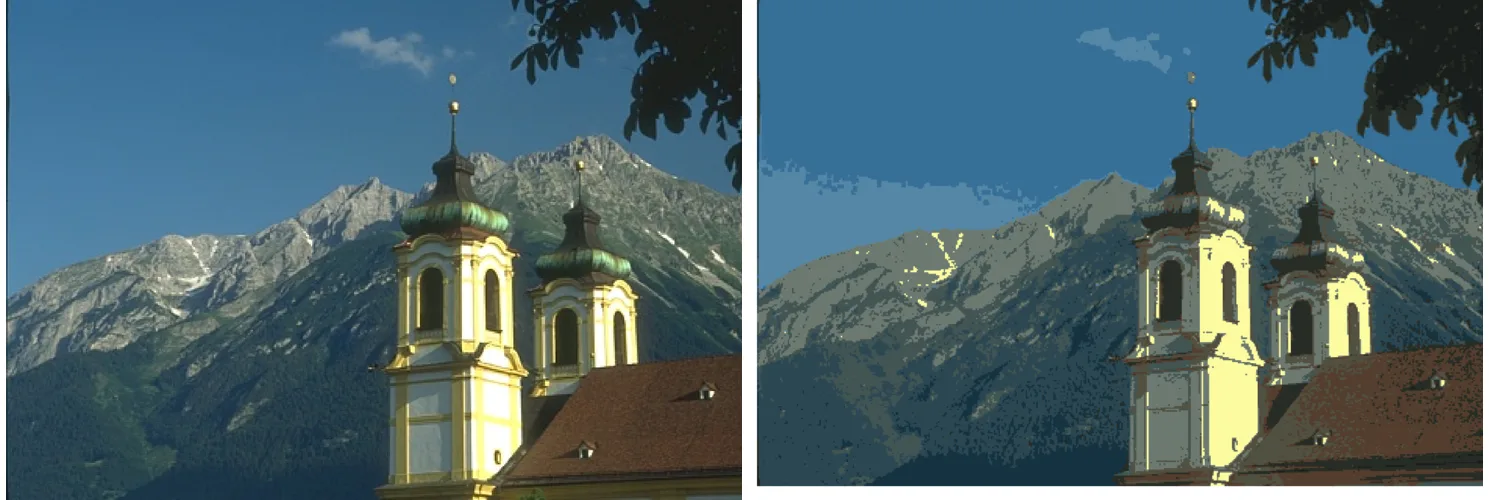
The report’s four-repo evaluation runs every algorithm on the same set of BSDS300 photos and discusses the results in §7.5. Here is its own default mean-shift run next to the source photograph, and a second example:
Figure 26, panels (a) and (b): the report’s own default run, .
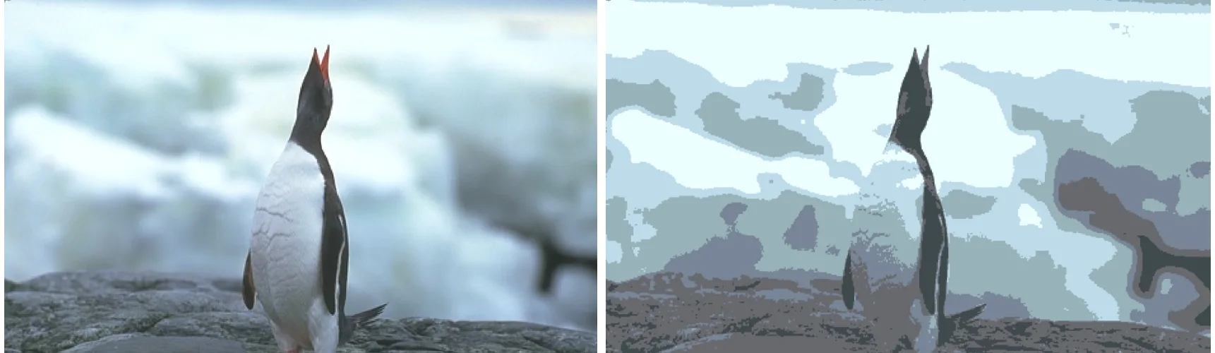
Figure 31: the blurred background gives mean shift a much noisier density surface than the church’s clean sky, and it shows.
The report’s own words on mean shift:
Finally the mean-shift algorithm created quite a few more regions than the rest of the algorithms. The slight increase in brightness at the edge of the mountain was enough to associate part of the sky with the clouds. Furthermore, there is also a clear separation between the top and bottom of the mountain with isolated patches for the snow. There are a few regions such as the trees which could have been better grouped.
That is exactly what step 4 predicts. A gradient sky is not one colour: it is a continuum, so a fixed radius slices it into as many bands as fit, and the “isolated patches for the snow” are precisely the connected-component check working as designed: scattered bright patches on the mountain either cohere into a real connected blob (kept) or do not (discarded, then reabsorbed into whatever region is nearest to them in colour, which is why they show up as small islands of the wrong region rather than vanishing). Unlike EM’s Gaussian-mixture fit, mean shift never has to be told how many regions to produce: the trade is that it also has no way to prefer fewer, larger ones. The radius is the only lever, and was tuned for one photograph’s histogram, not every photograph’s.
Where this sits among the three algorithms
Mean shift’s entire cost is data-dependent and, unlike EM’s fixed or normalised cuts’ fixed eigenproblem size, genuinely unbounded in advance: the peeling loop runs until the image runs out of dense clusters, which could be five iterations or fifty depending on how much of the photograph is flat colour. That is also its appeal. It is the only one of the three algorithms in this section that does not ask you, before you have looked at the picture, how many regions it contains.
Normalised cuts turns the same question into an eigenvalue problem instead, and gets its own post next.