Blog · Research infrastructure ·
A 2004 segmentation algorithm as a graph pooling layer
Felzenszwalb & Huttenlocher's merge rule, unchanged, driven by a learned edge metric instead of colour distance, so it coarsens a graph the way a neural network pools instead of the way a photograph gets segmented.
- interactive
- graph-neural-networks
- pooling
- felzenszwalb-huttenlocher
- pytorch
- research-infrastructure
Classical pooling downsamples on a fixed grid: a 2x2 max or average, applied everywhere, whether or not the four pixels underneath it have anything to do with each other. Post 69 reimplemented Felzenszwalb and Huttenlocher’s 2004 graph-based image segmentation from the paper and showed it is fast enough to run on a camera feed: sort every edge in a pixel graph by weight, walk the sorted list once, join two components whenever the edge between them is cheap relative to how varied each component already is. I am not reimplementing that here, and I am not re-deriving it either: post 69’s merge-rule module, untouched by this post, is reused exactly as it stands. What I did with it, in the masters research this post is drawn from, was put it to a different job: instead of segmenting a photograph, it coarsens a graph of feature vectors, which is what a pooling layer in a neural network needs to do. The merge rule does not change either way. What changes is the one number every merge decision depends on: the distance between two nodes.
The same merge rule, a different distance
Felzenszwalb and Huttenlocher’s threshold rule, exactly as post 69 derives it, merges two components and across an edge of weight when
Nothing about that rule cares what is measuring. Post 69’s merge-rule module sets
to the Euclidean distance between two pixels’ RGB values, because that is what
Felzenszwalb and Huttenlocher’s paper does for a photograph. PegbisPooling, the class I
built around a vendored copy of the same algorithm, sets to a learned distance
between two nodes’ feature vectors instead:
def forward(self, x, pos, edge_index, batch):
    e = (x[edge_index[0]] - x[edge_index[1]])**2
    e = torch.sqrt(e.matmul(self.weight.abs()/self.weight.abs().sum())+1e-10).view(-1)
x is the graph’s node features, one row per node; self.weight is one learnable scalar
per feature channel. I sat down to write this post half remembering that as a softmax
over the channel weights, the way an attention weighting usually gets normalised.
Rereading the actual line, it is not: self.weight.abs()/self.weight.abs().sum() is
plain L1 normalisation of the absolute value, no exponential in sight. It has the property
that matters for this post either way, every channel’s contribution stays non-negative and
the whole vector sums to one, so e is still a legitimate distance, just one whose
per-channel scaling gradient descent gets to set rather than a fixed 1 for every colour
channel and 0 for everything else. The widget below lets you set that vector by hand
instead of training it, which is the thing a reader can actually do with it.
That e, one score per edge, is the entire interface between “a distance a network
learned” and Felzenszwalb & Huttenlocher’s algorithm. Everything downstream of it,
sorting, the union-find, the per-component threshold, is segment_graph’s job (the
vendored, torch-tensor-flavoured port I did not write and do not reproduce here, see the
credit below), which is the exact same job felzenszwalb::segment_graph_into does for
post 69. The merge predicate does not know or care that e came from a learned weight
instead of sqrt((r1-r2)^2 + (g1-g2)^2 + (b1-b2)^2).
What the layer actually pools
A pooling layer has to do more than decide which nodes merge, it has to produce a smaller
graph the next layer can run on. __merge_edges__ does that part:
def __merge_edges__(self, x, pos, edge_index, batch, edge_score):
    cluster = segment_graph(edge_index.cpu(), edge_score.cpu(), x.size(0), self.cluster_c, self.min_size).to(x.device)
    new_x = scatter_mean(x, cluster, dim=0)
    new_pos = scatter_mean(pos, cluster, dim=0)
    new_batch = x.new_empty(new_x.size(0), dtype=torch.long)
    new_batch = new_batch.scatter_(0, cluster, batch)
    new_edge_index = knn_graph(new_pos, self.k, new_batch, loop=False, flow=self.flow)
cluster is Felzenszwalb & Huttenlocher’s output, a component id per node. scatter_mean
folds every merged group’s features and positions down to one row each, the pooled
node’s feature is the mean of everything that merged into it, its position is the mean
position too. A fresh k-nearest-neighbour graph gets rebuilt over the coarse node
positions, because the layer’s input was a point cloud with no fixed grid to fall back to,
knn_graph is doing the job the widget’s own coarse-graph panel does more directly below,
by drawing an edge between two pooled regions whenever the original graph had an edge
crossing between them.
There are two dated versions of this class in the repository, each named for the day I
started it. This post’s date comes from the second one’s own filename: both versions
landed in git on 2020-04-11, in one bulk import commit together with the first thirteen of
my own experiment scripts, so it is the date embedded in the filename I am trusting, not
the commit date. The February version merges with one symmetric threshold, the object’s
c attribute. The March version, quoted above, splits that into cluster_c (the merge threshold itself,
unchanged in meaning) plus ca, cb, alpha, beta, and adds a training signal for the
edge weight itself:
def lossfn(self, cluster, y, edge_score, edge_index):
    val_inst = y >= 0
    same_class_mask = (y[edge_index[0]] == y[edge_index[1]]) * val_inst[edge_index[0]] * val_inst[edge_index[1]]
    yi_eq_yj = edge_score[same_class_mask]
    yi_neq_yj = edge_score[torch.logical_not(same_class_mask)]
    topk = min(len(yi_eq_yj), len(yi_neq_yj), self.loss_top_k)
    return self.alpha*(yi_eq_yj.topk(topk, largest=True)[0] - self.ca).clamp(0).mean() + \
        self.beta*(self.cb - yi_neq_yj.topk(topk, largest=False)[0]).clamp(0).mean()
yi_eq_yj is the learned distance on edges whose two endpoints carry the same ground-truth
label, yi_neq_yj the same on edges that cross a class boundary. The loss pushes the
worst same-class edges below ca and the worst different-class edges above cb, an
auxiliary signal aimed squarely at the one thing this post is about: shaping what “close”
means before Felzenszwalb & Huttenlocher’s threshold ever sees an edge weight.
Wired in more than I remembered
That does not change the plain bottom line: no checkpoint, log, or accuracy number
survives for any of those seven scripts either, so I still cannot tell you whether it
worked. It does change the shape of the story. This was not a layer I wrote once and set
aside untested, it got a real three weeks of hand-tuned attention, stacked three deep in
a real model, before the graph U-Net that eventually did get trained end to end, the
subject of post 63, settled on a plainer, purely
distance-based PosEdgePool instead. An idea that got tried, more than
once, and was quietly dropped for something simpler, rather than one that never left the
drawing board.
Trying it on an image, since I have no point cloud to show you
Every cell of a small grid over the image (default 24 cells on the long side) gets a
4-channel feature vector: red, green, blue, and a texture channel, the magnitude of a
small Sobel gradient of luminance over the same grid. That grid is a graph, same 8-connected
neighbours the merge-rule module uses for pixels. Both panels pool it through the exact same
PegbisPooling formula, sqrt(sum((fi-fj)^2 . |weight| / sum|weight|)), computed by the
widget’s own edge_weight function. The “fixed colour distance” panel’s weight
is pinned at equal red, green, blue and zero texture the moment its handle is created and
never moves again, which is what recovers the classic, unweighted-feeling Felzenszwalb &
Huttenlocher metric post 69 already uses on full photographs as a special case rather than
a second implementation of it. The “shape the metric” panel’s weight is whatever its four
sliders currently say. Pushing all the weight onto texture and away from colour makes the
merge rule blind to a sky-and-mountain colour difference and sensitive only to how smooth
or detailed a patch is; pushing it back onto equal red, green and blue with texture at zero
makes the two panels’ edge weights identical, not just similar, because at that point they
are the same function fed the same weight vector. Nothing about the merge rule changes
between the two panels either way, the widget calls felzenszwalb::segment_graph_into
in both, only the weight vector its edge-weight function reads does.
Below the merge threshold and weight sliders sits a “reveal merges” slider. It does not
re-run a separate incremental version of the algorithm, segment_graph_into already sorts
its edges and only ever looks at ones already processed, so replaying it on a shorter
prefix of the very same sorted list gives back exactly the labels a full pass would have
had at that point. Scrubbing it back shows the grid as a lot of small, barely-merged
regions; scrubbing forward shows them coalescing exactly the way the sorted-edges,
one-pass argument post 69 makes says they must.
Each panel also draws its own pooled graph next to the original grid, not just a
recoloured image: one node per surviving region, placed at that region’s mean position,
sized by how many cells merged into it, connected to whichever other regions it still
shares a boundary with. That is scatter_mean and the coarse adjacency __merge_edges__
builds with knn_graph, done directly from the grid’s own edges since there is no
point cloud here to re-run a k-NN search over. A third panel pools the same starting grid
the way an ordinary CNN would, fixed square blocks, no notion of which cells actually
belong together, sized so its block count lands close to the graph panels’ own region
counts. Same input, same rough output size, one of them shaped by what is actually in the
image.
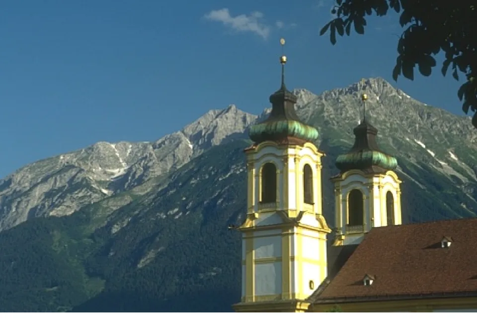
Post 69’s sample photograph, reused here as the widget’s bundled default.
With JavaScript on, this becomes a live widget: a small feature grid over this photo (or your own upload) gets pooled two ways, fixed colour distance and a weight you can shape across red, green, blue and texture, with a merge-reveal slider and each panel’s pooled graph drawn beside its starting grid. A third panel pools the same grid on a fixed block, for comparison.
The Rust side
The pooling code lives in a new module in segment-wasm, the same crate post 69’s
merge-rule module lives in. Both the union-find module (posts 35, 42) and the merge-rule
module itself are untouched: the new module just reuses felzenszwalb::segment_graph_into
for every merge, both the full pass and the “reveal merges” prefix replay, and adds
exactly what post 69’s module did not need: a multi-channel weighted edge builder, the
scatter_mean pooling, and the coarse adjacency. Ten new tests exercise it, including one
that checks the actual claim this post makes: with the same threshold k, the same pair
of nodes merges when the weight favours
their (small) colour difference and stays apart when it favours their (large) texture
difference, on a real computed edge weight rather than an assertion in prose. cargo test -p segment-wasm is 52 cases across the whole crate now, 10 of them new here, all passing.
The compiled module grew from about 137.9 kB to 147.1 kB, roughly 9 kB for this module.
Where this leaves it
No accuracy number exists for PegbisPooling anywhere I can find, on ScanNet or on
anything else. What does exist is a working, tested reuse of a 2004 algorithm as a
learned-metric pooling operator, three weeks of real (if never validated) training
attempts at it, and, in the graph U-Net that did eventually get trained end to end, a
decision to use something plainer instead. That last part is not a failure this post is
smoothing over, PosEdgePool’s job in post 63 is the
same merge-and-coarsen job this layer does, just without the learned metric, which is
itself evidence the metric-shaping idea was interesting enough to try and not, in the end,
the piece that made it into the architecture that got finished.