Blog · Features and preprocessing ·
Descriptors and the ratio test
Detecting a corner twice is the easy half. Recognising it again is the hard one: Lowe’s ratio test, a 5-pixel correctness threshold, and thirteen detector–descriptor pairs that mostly fail, rebuilt as a live oriented-FAST/rBRIEF matcher in Rust and WebAssembly.
- interactive
- feature-descriptors
- ratio-test
- brief
- hamming-distance
- rust
- wasm
Post 48 asked which corner detector finds the same physical point twice under a transformation. That turns out to be the easy half of the problem. Finding it twice tells you nothing if you cannot tell which point in the second image is the same one, and once I measured that, the answer was humbling: on the Bark sequence, under simultaneous zoom and rotation, thirteen detector–descriptor pairs score essentially 0%. On Wall, the single best pair manages 4.23%. This post is about why recognising a corner is so much harder than finding one, and about a benchmark that mostly reports failure, which, I think, is the useful thing about it.
The whole idea, in twenty lines
One throwaway script in the project, not part of the benchmark proper, is the clearest statement of the idea:
sift = cv2.xfeatures2d_SIFT.create()

kp1, des1 = sift.detectAndCompute(img1, None)
kp2, des2 = sift.detectAndCompute(img2, None)

bf = cv2.BFMatcher()
matches = bf.knnMatch(des2, des1, k=2)

good_matches = []
for m, n in matches:
    if m.distance < 0.7*n.distance:
        good_matches.append(m)
Detect keypoints in both images. Describe each one as a vector. For every descriptor in image 2, find its two nearest neighbours in image 1 by distance. Keep the match only if the best neighbour is convincingly closer than the second-best. That is the ratio test, and everything else in this post is either building the pieces it needs or measuring how well it works.
Detector and descriptor are two different jobs
They are usually named after the same paper, BRISK the detector and BRISK the descriptor, which makes it easy to forget they answer different questions. A detector finds a location: a corner, a blob, a point whose neighbourhood looks different from a shift of itself. A descriptor turns that neighbourhood into a vector that a different image’s neighbourhood, seen from a different angle or in different light, should land near. The report groups the descriptors this benchmark tests into four families:
- Local binary: BRISK, BRIEF, FREAK, LATCH, ORB, BOOST. Bit vectors from pairwise intensity comparisons: cheap to compute and cheap to compare.
- Spectra: SIFT, KAZE, AKAZE. Built from gradients and other continuous statistics of the patch.
- Basis-function: LUCID, DAISY. Built on a transform of the patch rather than a raw pixel test.
- Polygon-shape: descriptors built from a region’s own shape: area, perimeter, centroid.
The benchmark pairs each of thirteen descriptors with a detector to run under, and the pairing is not what you would guess:
detector_to_use = ["AKAZE", "BRISK", "KAZE", "ORB", "BRISK", "BRISK", "BRISK", "BRISK", "BRISK", "BRISK",
                   "SIFT", "SURF", "BRISK"]
feature_descriptors_to_test = ["AKAZE", "BRISK", "KAZE", "ORB", "BOOST", "BRIEF", "DAISY", "FREAK", "LATCH", "LUCID",
                               "SIFT", "SURF", "VGG"]
Only four descriptors run on their own namesake’s keypoints (AKAZE-AKAZE, BRISK-BRISK,
KAZE-KAZE, ORB-ORB, plus SIFT-SIFT and SURF-SURF). The other seven third-party descriptors,
BOOST, BRIEF, DAISY, FREAK, LATCH, LUCID and VGG, all describe BRISK’s keypoints, because
OpenCV’s xfeatures2d descriptors only compute a vector at a location; they do not detect
one. BRISK is the detector doing the work in nine of the thirteen rows of every table below,
which matters when you read them: a bad BRISK-X score can mean BRISK put the point somewhere
X could not describe well, not that X itself is weak.
Lowe’s ratio test
The idea, credited to David Lowe’s 1999/2004 SIFT paper, is that a genuinely distinctive
feature has one clear best match and a distant second-best; a repetitive texture (brick,
bark, a chain-link fence) has many similar candidates, so its best and second-best
distances are close together. The benchmark’s get_match_rate function applies it after a
brute-force match:
matches = matcher_alg.knnMatch(des1, des2, k=2)

correct_matches = []
incorrect_matches = []
for match_1, match_2 in matches:
    if match_1.distance < match_thresh * match_2.distance:
        ...
with match_thresh=0.75 as the default parameter. Written as an inequality on the two
nearest distances from one query descriptor:
This one line predicts, before you run a single trial, that Wall (brick) and Bark (rough bark texture, and zoomed and rotated on top of that) will be the two hardest datasets in the whole benchmark: every patch of brick or bark looks like every other patch of brick or bark, so and are close together and the ratio test throws almost everything away. The numbers below confirm it.
What counts as a correct match
A match surviving the ratio test still might be wrong: it just means the descriptor was
confident. Correctness needs ground truth, which is what the Oxford/VGG homographies
provide: a default thresh_sq = 25 is a 5-pixel threshold, squared, on the distance between
the matched keypoint in image 2 and where image 1’s keypoint should have landed.
kp_t_1_2 = np.dot(T_1_2, kp_1_np.T)
# seems they occasionally encode the light levels into this matrix too? Docs unclear
kp_t_1_2 = (kp_t_1_2 / kp_t_1_2[2]).T
kp_t_1_2_test = np.dot(T_1_2, kp_1_np.T).T
...
if (np.sum(np.square(kp_t_1_2[match_1.queryIdx, :2] - kp_2_np[match_1.trainIdx, :2])) < thresh_sq or
        np.sum(np.square(kp_t_1_2_test[match_1.queryIdx, :2] - kp_2_np[match_1.trainIdx, :2])) < thresh_sq):
    correct_matches.append(match_1)
A homography maps a homogeneous point by matrix multiplication and then divides through by
the third (homogeneous) coordinate to get back to pixels: that division is kp_t_1_2.
kp_t_1_2_test is the same multiplication without the division. The comment above it is
me noticing, mid-experiment, that the
provided H1to*p matrices sometimes behave as though they are not pure homographies (as if
a lighting scale factor has been folded into the matrix alongside the geometry), so the code
accepts a match as correct if it lands within 5 px under either interpretation. I still do
not know which of the two is “right” for any given file, and I did not know back then
either, so testing both rather than guessing was the unbiased way to handle it.
The measurement: Tables 9–16
Eight datasets, thirteen detector–descriptor pairs each, matched against ground truth across five image pairs (1→2 through 1→6) and averaged. This is the report’s actual measured data, transcribed straight from its own result pages, not this post’s widget, which uses a different descriptor entirely (see below).
Both numbers check out against the report exactly as quoted above, I re-read both source pages before writing this sentence. Table 16’s discussion draws its own conclusion from the full set of eight tables: “the three best performing feature detector/descriptor pairs were the SIFT-SIFT, AKAZE-AKAZE and BRISK-BOOST”, an aggregate judgement across all eight datasets, not just Wall, and it lines up with what the sortable table below shows once you flip through a few datasets: AKAZE-AKAZE and SIFT-SIFT are near the top everywhere, BRISK-LUCID and BRISK-BRIEF are usually near the bottom.
The sortable panel below the widget carries all eight tables in full: click a column header to re-sort. Bark and Wall are worth loading first; Leuven and UBC (the two easiest datasets, where the scene barely changes) are worth loading right after, for contrast.
The unpublished figures
Something the report never showed anyone: an appendix titled “Matched features with the Leuven dataset,” thirty-four pages of exactly this kind of correspondence figure, green lines for matches inside the 5-pixel threshold, red for matches outside it, one page per detector–descriptor pair. I found every other report page already embedded as an inline image somewhere in the project, except these ones: they sit behind an HTML comment that nobody ever uncommented. They are also, by a wide margin, the best-looking figures in the whole project, so here is the first one:
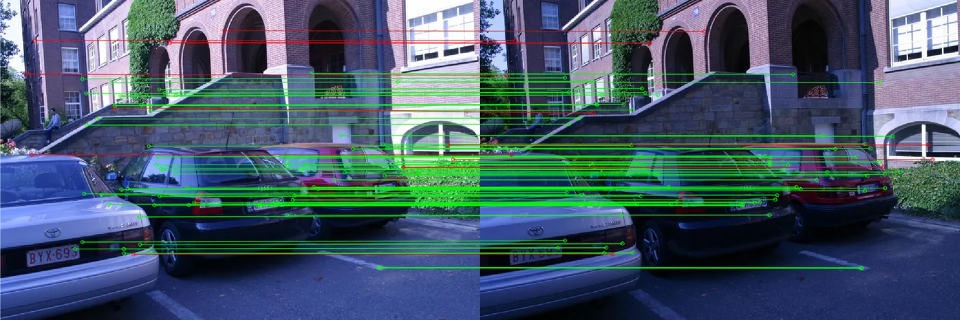
Figure 51 from the report’s unpublished appendix: AKAZE-AKAZE correspondences between Leuven images 1 and 2, mild lighting change, the easiest pair in the sequence. Never published before this post.
Match Bench
The widget below is a real, from-scratch feature matcher (oriented FAST keypoints, a 256-bit rBRIEF descriptor, and a brute-force Hamming matcher) running entirely in your browser via WebAssembly. Drag the ratio slider from 1.0 down toward 0.5 and watch which lines disappear first: the ones that were never confident hold on the longest, and the weak, ambiguous ones melt away fastest, because that is exactly what the ratio test is built to discard. No paragraph explains that as well as watching it happen.
Two things this widget is not. It is not a reproduction of Tables 9–16: those numbers came from OpenCV’s BRISK/AKAZE/SIFT and OpenCV’s own descriptors, benchmarked on real Oxford photographs against real homographies. This widget’s detector and descriptor are my own, smaller implementations (below), and, as the callout above says, its bundled images are report-page crops standing in for photographs I do not have. Think of Match Bench as the mechanism, live, and the tables above as the measurement; they are two different things pointing at the same idea, not the same experiment twice.
Where the green/red colouring comes from. With no homography to project through, correctness for the bundled Leuven pairs uses a substitute: because Leuven’s camera does not move (only the lighting does), a match is drawn green if it lands within an adjustable number of pixels of the same position in both images, and red otherwise. That is not the report’s geometric test; it is a reasonable stand-in for a sequence where the scene itself does not move, and the “consistency threshold” slider is the same kind of arbitrary 5-pixel cutoff as the report’s own, just exposed instead of hard-coded. Upload your own pair and that assumption stops applying: there is no reason to expect two arbitrary photos to align pixel-for-pixel, so uploaded matches are drawn in a single colour with no correct/incorrect claim at all.
With JavaScript on, this becomes a live matcher: pick a bundled Leuven pair or upload your own two photos, adjust the FAST threshold, drag the ratio-test slider and watch weak matches disappear, and browse Tables 9–16 as a sortable table beside it.
Oriented FAST, in brief
FAST tests sixteen pixels on a radius-3 circle around a candidate and asks whether at least nine consecutive ones are all brighter than the centre plus a threshold, or all darker than the centre minus it. It is cheap (most non-corner pixels reject after a handful of comparisons) but it says nothing about orientation, and a descriptor sampled without one breaks under rotation. “Oriented” FAST (Rublee et al., ORB, 2011) fixes that with the intensity centroid: sum and over a disk around the point, and take . A symmetric blob centres on itself and gets an arbitrary but stable angle; a real corner’s brighter or darker side pulls the centroid off-centre, which is exactly the direction a descriptor’s sampling pattern should be rotated to compensate for.
rBRIEF, but not OpenCV’s rBRIEF
A BRIEF descriptor is a set of pairwise intensity tests at fixed offsets from the keypoint: bit is 1 if the pixel at offset is dimmer than the pixel at , 0 otherwise. “Rotated” BRIEF (the r in rBRIEF) rotates every offset pair by the keypoint’s own orientation before sampling, so the same physical pattern of tests lines up the same way against the corner regardless of how the image is rotated.
Matching, and why the ratio slider is instant
Every descriptor in image A is compared against every descriptor in image B with a Hamming
distance: the number of differing bits, computed four u64 XORs and a hardware popcount
per pair, over up to 700×700 keypoints in a few milliseconds. The Rust side hands back the
best and second-best distance for every query and stops there; it does not apply the
ratio test itself:
pub fn match_bf(a: &[[u64; WORDS]], b: &[[u64; WORDS]]) -> Vec<(i32, u32, u32)> {
    a.iter().map(|qa| {
        let (mut best_idx, mut best_d, mut second_d) = (-1i32, u32::MAX, u32::MAX);
        for (j, qb) in b.iter().enumerate() {
            let d = hamming(qa, qb);
            if d < best_d { second_d = best_d; best_d = d; best_idx = j as i32; }
            else if d < second_d { second_d = d; }
        }
        (best_idx, best_d, second_d)
    }).collect()
}
The widget receives that flat (index, best, second) triple per query keypoint once, and
every tick of the ratio slider (or the consistency slider) just re-filters that array in
JavaScript (best < ratio * second) and redraws. Nothing gets re-detected or re-matched,
which is the only reason dragging the slider from 1.0 to 0.5 feels like a live picture
instead of triggering a fresh benchmark pass each time.
What the report concluded
Its own summary, in substance: feature descriptors are far from perfect, and making them work reliably in real conditions is genuinely hard. Having produced Tables 9–16, I do not think that reads as false modesty. A benchmark where the best score on an entire dataset is 4.23% is not a benchmark with a disappointing footnote, the footnote is the finding. Detectors (post 48) mostly did their job: BRISK alone still finds hundreds of keypoints under zoom, rotation, blur and viewpoint change. It is turning “a keypoint” back into “the same keypoint I saw a moment ago” that classical hand-crafted descriptors, on this evidence, are not very good at once the transformation gets large. That is the argument this benchmark makes, and reporting a wall of zeros rather than quietly picking an easier dataset is, I think, the more credible paper.