Blog · Camera geometry ·
Finding every corner on a checkerboard
An X-corner is a saddle point of intensity, so one threshold on the Hessian eigenvalues finds every corner in the image, plus a few thousand impostors. The rest of the algorithm is four geometric filters that know what a checkerboard is.
- interactive
- computer-vision
- camera-calibration
- corner-detection
- hessian
- wasm
cv2.findChessboardCorners returns a boolean. When it is True you get a beautiful
ordered list of sub-pixel corner positions and you get on with your life. When it is
False you get nothing, no reason, and no lever to pull.
I wanted to calibrate a camera from first principles, which meant I needed the correspondences from first principles too, which meant opening that box. The paper I worked from is Y. Liu et al. (2016), and its central observation is the sort of thing that makes an entire algorithm feel inevitable once you have heard it:
A checkerboard corner is a saddle point of image intensity. Walk along one diagonal through the crossing and you go dark → light → dark. Walk along the other and you go light → dark → light. The surface curves up one way and down the other, which is exactly what a saddle is. Unlike “corner-ness”, “edge-ness” or any of the other words we use for these things, a saddle has a crisp definition you can test at every pixel in one pass.
Everything after that is bookkeeping. Rewarding bookkeeping, because the first test finds every real corner and several thousand impostors, and the rest of the algorithm is four geometric filters that exploit what a checkerboard specifically is (centrosymmetric, gridded, right-angled) to delete them. Watching the count fall from a few thousand to exactly 156 is the most satisfying part of the whole thing, so there is a widget below that does exactly that.
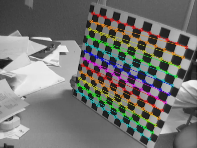
The output: 156 corners, found, filtered and then ordered into rows, which turns out to be the hard half.
The saddle test
Blur the image, take its second derivatives, and assemble the Hessian at every pixel:
At a saddle, : the two principal curvatures have opposite signs. You could hunt for negative local minima of the determinant directly, but the report points out you do not have to: the sign information is already in the eigenvalues, and for a symmetric 2×2 those have a closed form (Eq. 3.1):
so and is the saddle condition, one comparison per pixel, no neighbourhood search. In practice a bare sign test fires on noise, so Liu et al. ask for both eigenvalues to be a decent fraction of the strongest response in the image (Eq. 3.2), with the maximum of over the whole image:
The whole of that is nine lines of NumPy:
scaledimg = img_gray/255
rx = cv2.Sobel(scaledimg, cv2.CV_64F, 1, 0, ksize=7)  # Equivalent to gaussian blur and then derivative
ry = cv2.Sobel(scaledimg, cv2.CV_64F, 0, 1, ksize=7)  # Equivalent to gaussian blur and then derivative
rxx = cv2.Sobel(rx, cv2.CV_64F, 1, 0, ksize=1)
rxy = cv2.Sobel(rx, cv2.CV_64F, 0, 1, ksize=1)
ryy = cv2.Sobel(ry, cv2.CV_64F, 0, 1, ksize=1)

C_1 = rxx + ryy
C_2 = np.sqrt(np.square(rxx-ryy)+4*np.square(rxy))

lambda1 = 0.5 * (C_1 + C_2)
lambda2 = 0.5 * (C_1 - C_2)

max_l_1 = np.max(lambda1)

epsilon = C_val * max_l_1
corner_inc = np.where(np.logical_and(lambda1 > epsilon, lambda2 < -epsilon))
The comment on the Sobel lines is the load-bearing one. A 7-tap Sobel is separable into a
binomial smoothing kernel [1 6 15 20 15 6 1] one way and its difference
[-1 -4 -5 0 5 4 1] the other, so “blur then differentiate” is a single convolution and
the paper’s Gaussian pre-blur comes for free. The ksize=1 calls on the second line pair
are plain three-tap central differences, which is what OpenCV means by a 1-wide Sobel of a
first derivative.
One point per corner
The eigenvalue test fires on a blob around each crossing, not a single pixel, so the next step keeps only points that are the local minimum of the (blurred) determinant in their own 9×9 window:
surrounding_i = get_surrounding_pixels(corner_inc, 4)

S = cv2.GaussianBlur((rxx*ryy - rxy*rxy).astype(np.float32), (9, 9), 3)[surrounding_i]
curr_corners_i = corner_inc[0][np.where(np.argmin(S, axis=1) == 0)], corner_inc[1][np.where(np.argmin(S, axis=1) == 0)]
get_surrounding_pixels lays out the 81 window offsets with (0, 0) first, so
argmin(S, axis=1) == 0 means “the centre wins”, a neat way of writing a
non-maximum-suppression pass as one comparison per candidate with no explicit loop. On a
640×480 board photo this typically takes a few thousand threshold hits down to a few
hundred, and it is where the real corners stop being blobs and become points.
Filter 1: a checkerboard corner is centrosymmetric
Drop a disc of radius on a candidate and cut it into eight 45° sectors. If the candidate really is an X-corner, then sectors 180° apart sit in the same colour of square and should agree in mean intensity, while sectors 90° apart sit in opposite colours and should differ a lot. Six statistics capture that, built from the eight sector means in the function that builds the circular mask:
, , , are the should-agree numbers and want to be small; and are the should-differ numbers and want to be large. The test is a ratio, which is what makes it exposure-independent:
centro_sym_ind = np.where(np.logical_or(np.logical_and(D_1 < pD_3, D_2 < pD_3),
                                        np.logical_and(D_4 < pD_6, D_5 < pD_6)))
The logical_or is the clever bit and I did not appreciate it until I ported it. The first
group tests the sector pairs that straddle the axes; the second group
tests the pairs rotated 45°. Passing either is enough, which is what
lets a board photographed at 45° survive a mask whose sector boundaries are axis-aligned.
The function that builds the mask-offset table has my favourite line in the whole port:
angles = 180 * (np.arctan2(square_ind[0], square_ind[1]))
...
np.logical_and(angles <= np.pi * d1, angles > np.pi * d2)
Multiplying radians by 180 and comparing against degrees times π is a correct radians-to-degrees conversion with the division moved to the other side of the inequality. It is right. It took me a genuinely embarrassing amount of time to convince myself it was right.
Filter 2: a corner is never alone
Every interior corner of a board has at least three others close by. So:
ind_dist_constraint = np.where(np.count_nonzero(sq_dists < d_sq, axis=0) > 3)The > 3 rather than >= 3 is because the point’s own zero distance is in the count. This
is the filter that deletes isolated texture: a speck of dust, the corner of a monitor
bezel, one glint on a table edge.
Filter 3: the two nearest neighbours subtend a wide angle
For a real corner, the two nearest other corners lie along the board’s two axes, roughly 90° apart, so . For a false corner sitting in a little cluster of false corners, both neighbours are usually in the same direction and . Keep the ones below a threshold .
What makes this filter interesting is that it has to be iterated. Deleting a point changes its neighbours’ nearest neighbours, which can push them over the threshold too, so the pass repeats until a sweep removes nothing. On a messy image it takes three or four passes; on a clean one, one.
Where , , , come from
Four thresholds, all in pixels or ratios of pixels, all dependent on how big the board is in the frame. Hard-coding them would make the detector work at exactly one distance. The paper’s answer is lovely: build a histogram of every point’s nearest-neighbour distance, grow a window outward from the peak until it holds most of the data, take the mean and standard deviation inside that window, define , and derive everything from those (Eq. 3.3):
The board’s own pitch sets the scale, so the detector is scale-free by construction. Robust statistics doing real work.
Two more things are buried in that function, and both are archaeology rather than algorithm.
The annealing schedule is dead code. The same parameter function computes a factor
scale = 3 * (iter_max - iter)/iter_max and applies it to , so the
band was meant to tighten as the outer loop progressed. Both places that call it
pass a literal 0:
r, p, dsq, t = calculate_parameters(curr_corners_i, 0, max_iter, img_gray.shape)so scale is always 3 and the schedule never advances. It cost nothing and it does
nothing.
And C was supposed to tune itself. Sitting between the parameter code and the main
routine are two functions:
def decrease_c(current_c, was_decreasing, current_step):
    step = current_step if was_decreasing is None or was_decreasing else current_step/10
    return current_c - step, True, step


def increase_c(current_c, was_decreasing, current_step):
    step = current_step if was_decreasing is None or not was_decreasing else current_step/10
    return current_c + step, True, step
That is a bisection-with-backtracking search: walk in one direction while the candidate
count moves the right way, and cut the step by ten every time you overshoot and reverse.
Neither function is called anywhere in the repository. It is the fossil of an auto-tuner
that was abandoned in favour of the hand-tuned c_vals table, and it is the one piece of
this code I most wish past-me had finished, because it is precisely the weakness the
warning above admits to.
Ordering: the part nobody writes about
You now have exactly the right points and absolutely no idea which is which. A calibration solver needs corner of the image to correspond to corner of the physical board, so an unordered cloud is worth nothing.
Find the four extreme corners first (Eqs. 3.4–3.7; , are the coordinates of the -th corner):
which is the standard trick: the extremes of and are the corners of the bounding diamond, and for a quadrilateral that is not wildly rotated they are its top-left, top-right, bottom-left and bottom-right. Then walk one edge from to and the opposite edge from to , collecting the points that lie within a tolerance of each line and sorting them by distance along it. Pair them up, sweep a line between each pair, and each sweep hands back one row of the board in order.
The tolerance is itself derived from the data, 0.8 of the smallest gap between any two
surviving corners, and the “collect points near a line, sort along the line” primitive is
one function used three times. Two guards
make the whole thing refuse rather than guess: if the two edges come back with
different lengths it retries with the other pair of edges (a 90° rotation), and if any
swept row has a different length from the first, or the final grid is not the shape you
asked for, the function returns False instead of a plausible-looking wrong answer. Every
zero in Table 1 below is one of those returns firing.
Sub-pixel, and a bug
The last step nudges each integer corner to the intensity-weighted centroid of its neighbourhood (Eqs. 3.8–3.9, over a region around the corner):
The report says a circular region, “as this is rotationally symmetric and is, therefore, more robust”. The code uses a 9×9 square. It also weights by rather than . And then:
Isqr = img_gray[surrounding_i]
Isqr *= IsqrWatch the impostors die
Six of the datasets’ own frames are bundled, plus upload, drag-and-drop, paste and a camera button. Step through the pipeline and watch the count fall. The default is a dataset 2 frame (the set where this detector beat OpenCV) at the same the benchmark used. On that frame the chain runs 1 425 → 157 → 157 → 156 → 156 for a 13×12 board: the λ-test, then the local-minimum test, then centrosymmetry, distance and angle. Drop to 0.08 on the same frame and the first number becomes 4 835 and the last becomes 160, and the ordering refuses the answer because four impostors got all the way to the end.
(Those counts, and every count below that is not from Table 1, come from running my Rust port on the WebP the widget ships, not from the 2019 Python on the original TIFFs. They are the same algorithm on a re-encoded image, so they are close, not identical.)
With JavaScript on, this becomes a live corner detector: pick a board (or upload your own), then step through the saddle-response heat map, the eigenvalue threshold, the local-minimum test and the three geometric filters, with a running count of surviving candidates at each stage. Hovering a candidate renders the eight-sector centrosymmetry mask over it with its D-values. The ordered corner list downloads as JSON.
Things worth trying, in rough order of how much they teach:
- Push
Cdown. The threshold stage explodes (nearly 8 000 hits at on the default frame) and the filters start letting rubbish through. Push it up and real corners on the blurry side of the board vanish instead, and the ordering fails because a row is short. There is a window a few hundredths wide where it works, and finding that window by hand for every dataset is exactly what thec_valstable is. - Turn off “auto”. The four sliders are the adaptive values the histogram picked; drag
ddown and the distance filter starts eating the board’s own corners, because the neighbours are now further away than the threshold allows. - Hover the impostors on the “local min” stage (the ones out in the background) and look at the mask. On a real corner, and sit far below the threshold. On an edge, one of them jumps.
- Load dataset 6. It fails at every threshold, the way it failed in 2019. At the benchmark’s it dies early for want of candidates; nudge to 0.08 and it gets all the way to the ordering step before refusing. The next section explains what the printed cross in its top-left square is doing to it.
The JSON export is the input to the calibration post that follows, so the format is fixed:
format: "checkerboard-corners/v1", a board of cols × rows, and corners as a
row-major array of [x, y] pairs in image pixels, origin top-left: corner is board
column , row .
Results, including the interesting failures
Six of the seven datasets, hand-rolled detector against cv2.findChessboardCorners, over
the same frames. An image counts as identified only if the full ordered grid of the right
shape came out.
| Dataset | Images | Correctly identified | Identified by OpenCV |
|---|---|---|---|
| 1 | 52 | 52 | 52 |
| 2 | 25 | 10 | 4 |
| 3 | 15 | 15 | 15 |
| 5 | 15 | 10 | 15 |
| 6 | 10 | 0 | 9 |
| 7 | 7 | 7 | 7 |
Dataset 2 is the win. A 13×12 board, 156 corners, hand-held at some fairly severe angles. This detector found and ordered 10 of the 25 frames; OpenCV managed 4. I would love to claim insight here, but the likelier explanation is that OpenCV’s corner ordering is stricter than mine about heavily foreshortened boards, and the adaptive machinery happens to cope with the perspective gradient across a tilted board better than a fixed neighbourhood does.
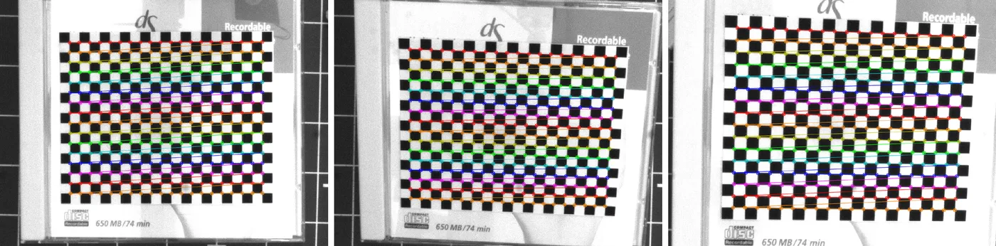
Figure 2 of the report: dataset 1, a 20×16 board on a CD case. 320 corners in each frame, all 52 frames, both detectors. When it works it really works.
Dataset 5 is where the noise gets in. The board is hand-held and there is a person standing right beside it. The report’s own words: the feature detector was not robust to all types of noise… where the persons ear got detected as a corner. An ear is, from a Hessian’s point of view, an extremely reasonable saddle point: the helix folds curve one way and the antihelix the other. It passes the eigenvalue test easily, and it is close enough to the board that the geometric filters have no reason to treat it as an outlier, which leaves it in the cloud that the ordering step has to make a rectangle out of. The report also notes a second cause on this set, less exotic and probably more common: there are also a few cases where the corner was too blurry to be detected. Ten of the fifteen frames still came through; five did not.
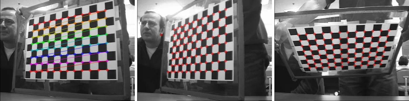
Figure 5: dataset 5. The board is hand-held with a person standing right beside it. Left: an ordered success. The other two: corners found, ordering refused.
Dataset 6 is a total loss, and it is my favourite result in the whole project. Zero frames out of ten, against OpenCV’s nine. The report is blunt about the cause: an interesting failure case can be seen in Fig. 6, where the cross in the checker-board corner lead the algorithm to fail.
The board in dataset 6 has a small printed cross inside its top-left square, a fiducial marker so a human can tell which corner is which. It is white, on black, and it fills most of that square.
I assumed the cross was being detected as a corner. Instrumenting the port let me check, and it is the opposite: the cross is not detected, and it takes a real corner down with it. Running my port on the bundled frame at , the pixel at the crossing nearest the marker passes the eigenvalue test (there is a fat blob of threshold hits sitting right on it) and then dies at the local-minimum step. The cross’s arms reach within a few pixels of that crossing and flood the neighbourhood with saddle response, and only one point per 9×9 window can win. Neither the marker nor the corner does.
So the board arrives at the ordering step with 88 points for an 88-corner board, but
they are not the right 88, because its top-left interior corner is missing and something
else has been promoted in its place. now lands one square along the top
edge, the walk down the “left” edge cuts diagonally across the board, and the two edges
come back different lengths. detect_checkerboard_corners returns False.
It fails at every threshold I tried, in three different ways: gives ragged rows, gives the mismatched edges above, and at (including the 0.1 the benchmark actually used) too few candidates survive to be worth ordering at all. Ten frames, zero successes, and the report’s one-sentence diagnosis was right about the cause even though I had the mechanism backwards.
The lesson generalises past this board. A marker designed to be maximally distinguishable to a human is, to a detector that only knows “saddle, centrosymmetric, gridded, right-angled”, indistinguishable from the thing it sits next to, and worse, it is loud enough to drown it out. OpenCV survives it because its ordering links the board’s own quadrilaterals into a mesh rather than trusting a handful of extreme points, so a single missing corner does not move the origin.
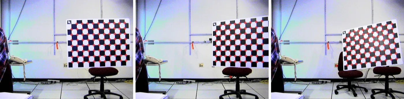
Figure 6: dataset 6. Nearly every corner is found and not one frame is ordered. The marker in the board’s top-left square is the reason.
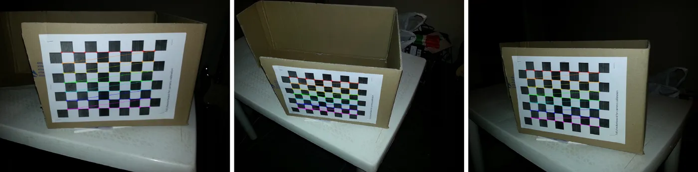
Figure 7: dataset 7, seven photographs from my own phone of a printed board taped to a cardboard box in a badly lit room. All seven. The adaptive parameters earn their keep here: nothing about this set matches the scale of the others.
What this does not do
Two things a reader would reasonably assume a calibration project does, and this one does not, stated up front so the next post can be read with the right expectations:
- There is no distortion model. The report is explicit: “Due to this, non-linear
distortions are not considered in this paper”, and the OpenCV benchmark deliberately
disables every distortion coefficient (
CALIB_FIX_K1…CALIB_FIX_K6plusCALIB_FIX_TANGENT_DIST) so the comparison is apples-to-apples. Nothing here undistorts anything. - Extrinsics are not recovered either. The planar method returns the intrinsic matrix and stops; the report lists this as a known drawback of the approach: “The draw back is that the extrinsic parameters of the camera cannot be fully recovered.”
Porting notes
The widget is a Rust port of the Python corner detector, compiled to WebAssembly (40.7 kB, no dependencies). Four places where it differs from the NumPy, all of them deliberate:
- No distance matrix. The NumPy builds a dense array of squared distances
and keeps re-slicing it, which is fine for a few hundred points and impossible for the
ten thousand candidates a low
Cproduces on a megapixel photo. The Rust answers the same two questions (“how many neighbours within ”, “which two are nearest”) against a uniform bucket grid. Same answers, linear memory. I²inf64, not wrapped inuint8, per the bug above.- The nearest-neighbour selection in the angle filter is written directly rather than
through the original’s
np.where-inside-a-fancy-index, per the warning above. - Manual parameters stay manual. The original always re-derives from the histogram at the end of every outer iteration; when you switch “auto” off in the widget, the four values you set are held fixed. The original has no manual mode at all: that control exists so you can break the thing on purpose.
The Sobel kernels, the reflect-101 border handling, the 9×9 σ=3 Gaussian on the
determinant, the eight-sector mask boundaries, the > 3 in the distance filter and every
one of the ordering guards are reproduced exactly, because the point of a port is to
reproduce the behaviour you are writing about, deviations included.
Next: what all these corners are actually for, recovering a camera’s intrinsic matrix from nothing but a plane you can print, using Zhang’s method and no OpenCV. That post takes the JSON above as its input.