Warping pixels: affine transforms and the interpolation you forgot about

cv2.warpAffine(img, M, size) is one line, and it hides two entirely separate decisions. The first is where each output pixel comes from: that is the matrix, and the surprise is that it gets applied backwards. The second is what value to give a pixel when “where it comes from” lands at $(148.37, 92.06)$ and there is no pixel there. The first section of my image-processing report is about the first decision; the second section, which is three paragraphs long and which I have thought about far more often since, is about the second.

This post is the affine chapter of that report (§2 and §3), rebuilt so you can drag it. The five matrices are transcribed from the report; the inverse mapping and the samplers are ported from BuildingBlocks/AffineTransforms.py and BuildingBlocks/Interpolation.py into Rust, so the arithmetic on this page is the arithmetic the post is describing rather than a call into a library.

The general form

An affine transformation maps points from one affine space to another and preserves points and parallel lines: a square can become any parallelogram, but it cannot become a trapezium. Written in homogeneous coordinates it is a single matrix multiply, which is the whole reason for the extra 1: translation is not a linear map, but it is a linear map one dimension up.

\begin{pmatrix} \mathbf{x}' \\ 1 \end{pmatrix} = \begin{pmatrix} \mathbf{A} & \mathbf{b} \\ \mathbf{0}^T & 1 \end{pmatrix} \cdot \begin{pmatrix} \mathbf{x} \\ 1 \end{pmatrix} \tag{2.1}

$\mathbf{A}$ is the $2 \times 2$ linear part (scale, rotation, shear, reflection, and every product of them), and $\mathbf{b}$ is the translation. Everything that follows is one particular filling-in of those six numbers. The report notes that affine transforms work in any number of dimensions; two is enough for images and is all I ever used.

Scale

\begin{pmatrix} \mathbf{x}' \\ 1 \end{pmatrix} = \begin{pmatrix} s_x & 0 & 0 \\ 0 & s_y & 0 \\ 0 & 0 & 1 \end{pmatrix} \cdot \begin{pmatrix} \mathbf{x} \\ 1 \end{pmatrix} \tag{2.2}

Values above one enlarge, values between zero and one shrink, $s_x = s_y = 1$ is the identity, and a negative value flips the image about that axis. That last one is worth remembering: flipud and fliplr are not special functions, they are $s_y = -1$ and $s_x = -1$ with the appropriate translation to bring the result back onto the canvas.

Translate

\begin{pmatrix} \mathbf{x}' \\ 1 \end{pmatrix} = \begin{pmatrix} 1 & 0 & d_x \\ 0 & 1 & d_y \\ 0 & 0 & 1 \end{pmatrix} \cdot \begin{pmatrix} \mathbf{x} \\ 1 \end{pmatrix} \tag{2.3}

The dullest of the five, and the most useful, because it is how you change the origin of any of the others.

Rotate

\begin{pmatrix} \mathbf{x}' \\ 1 \end{pmatrix} = \begin{pmatrix} \cos\theta & \sin\theta & 0 \\ -\sin\theta & \cos\theta & 0 \\ 0 & 0 & 1 \end{pmatrix} \cdot \begin{pmatrix} \mathbf{x} \\ 1 \end{pmatrix} \tag{2.4}

A rotation about the origin, which for an image means about the top-left corner, which is almost never what you want. Rotating about an arbitrary point $\mathbf{o}$ is the three-matrix sandwich $T(\mathbf{o}) \cdot R(\theta) \cdot T(-\mathbf{o})$ : shift the point of interest to the origin, rotate, shift back. The Python writes it out inline rather than as three matrix multiplies, but it is the same thing.

Shear

\begin{pmatrix} \mathbf{x}' \\ 1 \end{pmatrix} = \begin{pmatrix} 1 & s_x & 0 \\ s_y & 1 & 0 \\ 0 & 0 & 1 \end{pmatrix} \cdot \begin{pmatrix} \mathbf{x} \\ 1 \end{pmatrix} \tag{2.5}

Shear turns parallel diagonal lines into parallel vertical or horizontal ones, which is why it is the crude first fix for a photograph taken from the wrong angle. $s_x$ slides $x$ along in proportion to $y$ ; $s_y$ slides $y$ in proportion to $x$ . In the code these are called shear_h and shear_v, in that order, and their naming causes trouble later in this post.

Why the map runs backwards

Here is the part that the matrices alone do not tell you. You have the map, you have the source image, and you want the output image. The obvious thing (take each source pixel, push it through the matrix, write it where it lands) is wrong, and it is wrong in a way that is easy to see with the simplest transform there is.

Scale a $4 \times 4$ image by $1.5$ . The output is $6 \times 6$ , so it has 36 pixels. The source has 16. Sixteen values pushed into thirty-six slots leaves twenty slots empty, and they are not empty in a tidy border, but scattered through the image as a lattice of holes:

Scaling a 4 × 4 image by 1.5. Left: forward mapping fills 16 of the 36 output pixels and leaves 20 holes. Right: inverse mapping asks every output pixel where it came from, so all 36 get a value, but the place it came from is between source pixels, which is the whole problem of the next section.

You could paper over the holes afterwards (splat each source pixel as a small blob, or interpolate the scattered result), but you would still have the opposite problem when the map shrinks, where several source pixels compete for one output slot and you need some rule for who wins. Turn the whole thing around and both problems vanish. Iterate the output raster, push each output pixel through the inverse matrix into source space, and sample there. Every output pixel is visited exactly once and gets exactly one value, by construction. The price is that the coordinate you land on is fractional, and that price is section 3.

Every one of the five functions in AffineTransforms.py is written this way, and you can see it in the code without knowing what the code does. scale_image, lines 11–14:

region_x, region_y = np.meshgrid(
    np.arange(x_range[0], x_range[1], 1.0/scale_vector[0], dtype=np.float32),
    np.arange(y_range[0], y_range[1], 1.0/scale_vector[1], dtype=np.float32))

return interpolation_func(src, region_x, region_y)

The step is $1/s$ , not $s$ . Doubling the image means stepping through the source in halves, which is what “for each output pixel, where did it come from” means when the transform is a scale. translate_image (lines 26–27) subtracts the translation instead of adding it, for the same reason. And rotate_image (lines 41–45) evaluates Eq 2.4 directly on the output grid:

theta_rad = np.deg2rad(theta)
nx = np.cos(theta_rad)*(region_x - origin[0]) + np.sin(theta_rad)*(region_y - origin[1]) + origin[0]
ny = - np.sin(theta_rad)*(region_x - origin[0]) + np.cos(theta_rad)*(region_y - origin[1]) + origin[1]

return interpolation_func(src, nx, ny)

(region_x, region_y) is the output grid; (nx, ny) is where in the source to look. The “shift to the origin, rotate, shift back” sandwich is the - origin[…] and + origin[…] either side of it.

Where does the output canvas go?

Inverse mapping decides what to sample, not how big the canvas is. Every one of the Python’s functions defaults its output raster to the source’s own extent:

if y_range is None:
    y_range = 0, len(src)
if x_range is None:
    x_range = 0, len(src[0])

so by default a rotation or a shear crops itself against the original frame. For the shear figures the report works out the correct extent first, in get_shear_borders, lines 48–55:

def get_shear_borders(src, shear_h: float=0, shear_v: float=0):
    x1 = float(len(src[0]))
    x2 = len(src)*shear_h
    x3 = x1+x2
    y1 = len(src[0])*shear_v
    y2 = float(len(src))
    y3 = y1+y2
    return (min(x1, x2, x3, 0.0), max(x1, x2, x3)), (min(y1, y2, y3, 0.0), max(y1, y2, y3))

That is the four corners of the image pushed forward through Eq 2.5: $(0,0)$ , $(w, 0)$ , $(0, h)$ , $(w, h)$ become $(0,0)$ , $(w, s_v w)$ , $(s_h h, h)$ and $(w + s_h h, s_v w + h)$ , with the minimum and maximum of each coordinate taken. It generalises to any affine map in one line, and the Warp Bench below does exactly that: tick fit canvas to the warped bounds and the output raster is the bounding box of the transformed corners; untick it and you get the Python’s default behaviour, which is to crop.

The shear determinant

The pretty piece of algebra in the file is in shear_image, lines 67–74:

# nx = region_x + shear_v*region_y
# ny = shear_h*region_x + region_y

Dnx = region_x - shear_h * region_y
Dny = region_y - shear_v * region_x
D = 1 - shear_h * shear_v

return interpolation_func(src, Dnx/D, Dny/D)

The two commented-out lines are the forward map; the three live lines are its inverse, done by hand. Inverting a $2 \times 2$ is swap the diagonal, negate the off-diagonal, divide by the determinant, and for Eq 2.5 the determinant is

D = \det\begin{pmatrix} 1 & s_h \\ s_v & 1 \end{pmatrix} = 1 - s_h s_v,

\begin{pmatrix} 1 & s_h \\ s_v & 1 \end{pmatrix}^{-1} = \frac{1}{1 - s_h s_v}\begin{pmatrix} 1 & -s_h \\ -s_v & 1 \end{pmatrix},

which is exactly (x - s_h·y)/D and (y - s_v·x)/D. It is easy to forget the division: plenty of shear code just negates the off-diagonal term and calls it done, and for small shears you barely see the error, because $D \approx 1$ . At $s_h = s_v = 0.5$ , $D = 0.75$ and the picture is a third too small in both directions. At $s_h s_v = 1$ , $D = 0$ and there is no inverse at all: that transform squashes the whole plane onto a line, so asking where an output pixel came from has no answer. The Warp Bench prints $D$ next to the matrix, and says so when you drive it to zero.

Caveat

I found this while porting shear_image. The two commented-out lines have shear_h and shear_v the other way round from the three live ones. The live code inverts the matrix with $s_h$ in the top row and $s_v$ in the second; the comment describes the map with those two swapped. The comment is dead code so nothing was ever broken, it just reads wrong if you go through the file top to bottom.

The same mix-up reaches the figures too, and it took a second pass to catch. In Create_Building_Block_Images.py line 104, shear_image(T, 0.3, 0) (which sets $s_h$ , slides $x$ along with $y$ , and makes the image wider) is assigned to a variable called fig0236_a_shear_v, and line 106’s vertical shear is called ..._shear_h. My own Figure 4 in the report inherited the mix-up: panel (b) is labelled “Vertical Shear” and panel (c) “Horizontal Shear” when they are the other way about. The maths and the images are both right, only the words are wrong. The Warp Bench’s s_h and s_v sliders follow Eq 2.5 and the live code, so Fig 4(b) there sets $s_h = 0.3$ and produces the wider image the report prints as its panel (b).

Interpolation, which is the interesting half

So the inverse map has told you that output pixel $(x', y')$ came from source position $(148.37, 92.06)$ . There is no pixel there. There are four pixels around it. The report gives the two standard answers.

Nearest-neighbour is “round to the nearest integer”. It is one operation, it never invents a value that was not in the source (which matters if your image is a label map or a mask, where the average of “road” and “sky” is meaningless), and it produces a visibly pixelated result on anything else.

Bilinear is a weighted average of the four surrounding pixels. Define the fractional parts

r_x = x - \lfloor x \rfloor, \qquad r_y = y - \lfloor y \rfloor,

then four weights,

w_1 = 1 - r_x, \qquad w_2 = r_x, \qquad w_3 = 1 - r_y, \qquad w_4 = r_y \tag{3.1}

and the interpolated value is their product-weighted sum over the four corners:

\begin{aligned} I(x, y) = \; & w_1\big(w_3 I(\lfloor x \rfloor, \lfloor y \rfloor) + w_4 I(\lfloor x \rfloor, \lfloor y \rfloor + 1)\big) \; + \\ & w_2\big(w_3 I(\lfloor x \rfloor + 1, \lfloor y \rfloor) + w_4 I(\lfloor x \rfloor + 1, \lfloor y \rfloor + 1)\big) \end{aligned} \tag{3.2}

Written that way it is obviously separable: the inner brackets are two linear interpolations down the $y$ axis, and the outer sum is one linear interpolation across them in $x$ . Do it in the other order and you get the same number, which is where the “bi” comes from. The four products $w_1w_3, w_1w_4, w_2w_3, w_2w_4$ sum to one, so the result never leaves the range of its four inputs (no overshoot, unlike bicubic), and at an integer coordinate $r_x = r_y = 0$ , the weights collapse to $(1, 0, 1, 0)$ and you get the pixel itself. The identity warp really is the identity, under either sampler; there is a unit test that says so.

Here is that written out in the port, from wasm/crates/imaging-wasm/src/warp.rs:

let fx = x.floor();
let fy = y.floor();
let rx = x - fx;
let ry = y - fy;
let (w1, w2, w3, w4) = (1.0 - rx, rx, 1.0 - ry, ry);
let (x0, y0) = (fx as isize, fy as isize);
let p00 = tap(src, sw, sh, x0, y0, clamp);
let p01 = tap(src, sw, sh, x0, y0 + 1, clamp);
let p10 = tap(src, sw, sh, x0 + 1, y0, clamp);
let p11 = tap(src, sw, sh, x0 + 1, y0 + 1, clamp);
let mut out = [0.0f32; 4];
for k in 0..4 {
    out[k] = w1 * (w3 * p00[k] + w4 * p01[k]) + w2 * (w3 * p10[k] + w4 * p11[k]);
}

Credit

In the original repo this is not my code at all. BuildingBlocks/Interpolation.py is two functions and nine lines, and both of them are wrappers:

def nearest_interpolation(src, x_coords, y_coords):
    return cv2.remap(src, x_coords, y_coords, cv2.INTER_NEAREST)


def linear_interpolation(src, x_coords, y_coords):
    return cv2.remap(src, x_coords, y_coords, cv2.INTER_LINEAR)

The maths of Eq 3.1 and 3.2 is in the report; the arithmetic in the repo is OpenCV’s. Everything above the sampler (the meshgrids, the inverse maps, the determinant division, the border calculation) is mine. The Rust in this post is a fresh implementation of the two lines OpenCV was doing, written so that the page can show you the difference between them; I have not diffed it against cv2.remap pixel for pixel, and I would expect the odd grey level of disagreement at edges.

What nearest-neighbour actually costs

The report’s Figure 6 is the payoff of the whole chapter: a 50 × 50 crop of the same rotated letter, sampled both ways and blown up so you can see individual pixels. Here is that figure regenerated with my own letter T (rotated 21° about its centre, cropped at the same size, magnified 6×) using the Rust above rather than OpenCV:

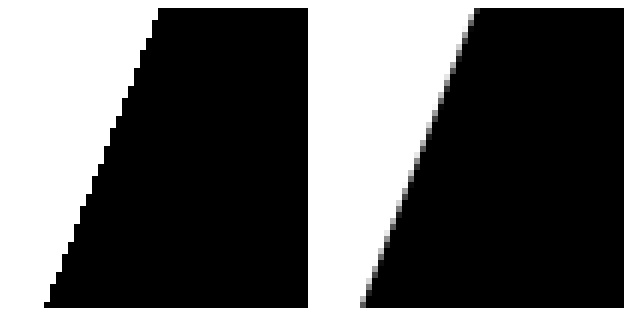
Two magnified 50 by 50 crops of the same rotated letter edge. On the left, nearest-neighbour: the diagonal boundary between white and black is a hard staircase of square blocks. On the right, bilinear: the same boundary is a smooth ramp, one or two pixels wide, of intermediate greys. — A reproduction of report Figure 6 (p. 8): nearest-neighbour on the left, bilinear on the right, on the same 50 × 50 block of a letter T rotated by 21°. The original figure used a Gonzalez & Woods plate; this one uses a letter T I drew, so the picture is mine but the experiment is the report’s.

Nearest-neighbour turns a straight diagonal into a staircase. Bilinear turns it into a one- or two-pixel ramp of intermediate greys: it has invented values that were not in the source, which is precisely what makes the edge look straight. Neither is “correct”: the source has no information about what is between its pixels, and the two samplers are two different guesses. Nearest guesses that the image is piecewise constant. Bilinear guesses that it is piecewise linear. Real edges are neither, and that is why there is a whole literature past this point.

The staircase also tells you how much a rotation costs you even before you look at the values: rotate an image by 21° and rotate it back, and you do not get the original. Each pass resamples, each resample loses a little, and with nearest-neighbour it loses in a way that compounds: try it in the widget, twice through $+21°$ and $-21°$ , and compare the two samplers.

The Warp Bench

Everything above, live. Pick a picture (the built-in letter T, the report’s characters test pattern, a drawing, an upload, or your camera) and drag the five parameters. Three things to do with it:

Move the pointer over the output. The two panels underneath show the same 50 × 50 block of output pixels sampled both ways, pixel-doubled: report Figure 6, wherever you happen to be pointing. Park it on a near-vertical edge of the letter and drag $\theta$ slowly; the staircase on the left reorganises itself in jumps while the ramp on the right slides smoothly.

Press the report-figure buttons. They set the sliders to the exact arguments in Create_Building_Block_Images.py, so the widget reproduces the report’s figures rather than something that looks like them:

Report figure	Driver line	Call
Figure 1, scaling	66	`scale_image(T, (4, 4))`
Figure 2, translation	121	`translate_image(T, (60, 20))`
Figure 3, rotation	82	`rotate_image(T, 21, centre)`
Figure 4(b)	104	`shear_image(T, 0.3, 0)`
Figure 4(c)	106	`shear_image(T, 0, 0.3)`
Figure 5	108	`shear_image(test_pattern, 0.1, 0.4)`

Watch the matrix. The panel beside the canvas prints the composed $3 \times 3$ of Eq 2.1 as you drag, and the toggle swaps it for the inverse: the matrix that is actually evaluated, once per output pixel. The dashed outline on the canvas is where the source frame lands; the cross is the rotation origin, which you can move by clicking, and the box is the magnifier.

Report Figure 6 reproduced: a rotated edge sampled with nearest-neighbour on the left and bilinear on the right — InteractiveWarp Bench

A few things worth trying. Set the scale to ×4 with nearest selected and look at the magnifier: every source pixel has become a hard 4 × 4 block, which is the honest picture of what “no information between the samples” means. Switch to bilinear and the same blow-up becomes a smooth ramp: no more information, but a much more plausible guess. Then push $s_h$ and $s_v$ toward $0.9$ each and watch $D = 1 - s_h s_v$ fall toward $0.19$ while the picture inflates by the reciprocal; nudge them to 1.0 and the transform has no inverse and the bench says so.

Untick fit canvas to the warped bounds to get the Python’s default framing, where the output raster is the source’s own size and a rotation throws its own corners away. And clamp edges swaps the transparent border for edge replication, which is the difference between BORDER_CONSTANT and BORDER_REPLICATE in OpenCV’s vocabulary.

Credit

The driver scripts in this repo read their inputs from ../Datasets/DIP3E_Original_Images_CH02/ and …_CH03/: the companion image set for Gonzalez & Woods, Digital Image Processing, 3rd edition. Those plates are not committed to the repo and never should have been; they are freely downloadable from imageprocessingplace.com, and without them Create_Building_Block_Images.py prints “Could not find image at:” and exits. Every figure in the report was rendered before that, so nothing here is blocked by it, but you cannot re-run the scripts as they stand without the download.

The letter T on this page is one I drew, not the plate. The characters test pattern in the bench is Fig0237(a)(characters test pattern) as it was rendered into the report’s own Figure 5, and it is Gonzalez & Woods’.

What I would change

The thing I would do differently is not in the maths, it is in the interface. Every function in AffineTransforms.py takes its own parameters and builds its own coordinate grid, so composing two transforms means resampling twice, and resampling twice through nearest-neighbour is visibly worse than resampling once through the composed matrix, because each pass quantises the error the previous one made. The right shape is the one the widget uses: build the $3 \times 3$ , compose as many as you like by multiplying, invert once, resample once. That is four lines of numpy and it would have made the shear determinant unnecessary, because a general $2 \times 2$ inverse divides by the determinant anyway.

The second thing is that the whole chapter treats interpolation as a two-option menu, and the interesting question is the one neither option asks: what is the image between its samples? Nearest says a staircase, bilinear says a tent. Ask instead what band-limited signal the samples came from and you get sinc, and Lanczos, and the whole resampling literature, and also the reason why bicubic sometimes shows a bright halo along a sharp edge, which is overshoot from a kernel that, unlike bilinear, is allowed to go negative. That comes later in this series, in the frequency-domain post, where the aliasing that resampling causes gets its own figure.